Introduction

Wave buoys represent a prevalent means for in situ measuring sea surface wave characteristics in both the world’s oceans [1, 2] and the Russian seas [3, 4]. The operational principle of wave buoys is based on tracking the motion of a floating body assumed to perfectly follow the sea surface [5]. The measurement of motion can be achieved through various methods, all of which are generally based on two primary types of measurements: inertial measurements (typically include measurements of the geomagnetic field) [5, 6] and global navigation satellite system (GNSS) measurements [7–9]. This paper focuses on the first type of measurements due to the progress in microelectromechanical systems (MEMS) over the past few decades. The development of MEMS has led to the widespread availability of inertial motion units (IMUs), which have become increasingly attractive due to their low cost, lightweight, compact size, energy efficiency, and immunity to radio interference when compared to analogous GNSS-based sensors.

In the early versions of wave buoys, the IMU measured linear acceleration along the vertical direction [10]. To stabilize the vertical axis, mechanically damped gimbals were used, thereby providing a direct estimate of the vertical accelerations of the hull. Consequently, this approach resulted in a non-directional elevation spectrum, significant wave height (SWH), and the period of dominant waves [1, 11]. When combined with magnetic sensors, such systems are capable of tracking the hull tilt with reference to the magnetic north, enabling the estimation of directional wave spectra.

With the development of MEMS technologies, the use of inertial sensors rigidly attached to the hull, often referred to as strapped-down IMUs, has become more suitable for wave measurements [12, 13]. The lack of mechanical stabilization is compensated by the simultaneous measurement of three components: acceleration (accelerometer), rotation rate (gyroscope), and geomagnetic field (magnetometer).

In theory, given the initial conditions are known, these measurements are sufficient to unambiguously determine the position and orientation of the hull, which is necessary to calculate the wave parameters. However, the presence of noise makes the estimation of the hull orientation unreliable due to the accumulation of errors over time. It should be noted that this is a standard navigation problem, the solution of which is especially important for unmanned aircraft technology, robotics, entertainment industry, etc. 

The early strapped-down navigation systems used an approach based on the ability to estimate orientation using two reference vectors [14, 15], such as the gravity vector and the geomagnetic field. This deterministic approach was called the TRIAD method, since the rotation matrix determining the orientation of a body in a fixed reference frame is a combination of three vectors, two reference vectors and their cross product. The main drawback of the TRIAD method is the errors associated with the distortion of the gravity vector by inertial forces arising due to the accelerated motion of the moving reference frame.

Today, the traditional solution for wave buoys is a recursive Kalman filter [16–18], aimed at assimilating all possible types of measurements to estimate the true orientation of the sensor, its acceleration, velocity, and position in a fixed reference frame [6, 18–27].

The Kalman filtering provides a weighted estimate of the current state of a dynamic system based on the previous state history and current measurements, the process also known as “data fusion”. The choice of weighting factors depends on the estimated measurement errors. This approach is useful when a series of generally “precise” measurements is interrupted by “erroneous” readings. In the case of inertial measurements, the “precise” measurements can be obtained for uniform rectilinear (non-accelerated) motion. The “erroneous” measurements occur during accelerated motion of the sensor, when the measured gravity vector is distorted by additional inertial forces. A typical example of such a system is a vehicle that generally moves uniformly but experiences interruptions due to accelerations/stops and course changes. When measuring waves, the gravity vector is always distorted by inertial forces, since the buoy continuously follows the orbital motion of the surface waves. Therefore, the efficiency of using standard IMU data assimilation algorithms for wave measurement seems unclear.

This paper analyzes the errors that can potentially occur in wave measurements using conventional commercially available IMUs. This issue is important because the possibility of using simple and cheap sensors in wave buoys allows to create expendable buoy fleets for specialized scientific experiments that are unrealistic with traditional buoys due to their much higher cost [28]. On the other hand, the use of small sensors allows a significant miniaturization of the buoy hulls, thus extending their bandwidth to shorter waves, which are important for several geophysical applications. 

This study considers the noise characteristics of typical IMUs. Various methods for estimating buoy motion are analyzed, including a standard algorithm using the Kalman filter, as well as earlier methods based on the TRIAD method. The differences in the algorithm performance are demonstrated using the field data obtained from a wave buoy prototype. To illustrate the characteristics of the algorithms, a numerical simulation of an idealized buoy motion (the buoy that perfectly follows the waves) is performed. For the sake of brevity, we focus only on the retrieval of omnidirectional spectra and their two basic integral parameters, SWH and peak frequency, leaving the discussion of directional wave properties to other studies.

Materials and methods

General considerations. Let us consider a free-floating body perfectly following the local slope of the sea surface. The height of the wave ζ  is given by a plane sinusoidal wave ζt,x=AsinΩt+Kx , where A is the wave amplitude, Ω=2π is the radial frequency of the wave, F is the wave frequency, K is the wave number, x is the spatial coordinate, t is the time (Fig. 1). Usually, the most interesting wave parameter is the amplitude A, which cannot be obtained directly from the measurement of acceleration, rotation rate or magnetic field (combined accelerometer/gyroscope/magnetometer).

In the moving sensor reference frame x'y'z', the deviation of the measured magnetic field vector from the x'-axis can be interpreted as the local slope of the sea surface ξ=∂ζ∂x . The gyroscope readings corresponding to the rate of rotation around the y'-axis represent the rate of the slope change, η=∂2ζ∂x ∂t . The acceleration along the moving z'-axis is equal to the vertical acceleration in the fixed reference frame modified by the acceleration due to gravity, g=9.8  m/s².

Therefore,

g'=∂2ζ∂t2+g,                                      (1)

since the vector measured by the accelerometer is always normal to the surface. Indeed, the vector change of a stationary accelerometer reading, g⋅ez , is equal to the centrifugal acceleration of the sensor, AΩ2sinθ⋅ex+cosθ⋅ez , where θ  is the wave phase, and ex,ey,ez  are the unit vectors of the fixed reference frame. Obviously, the maximum tangent of the angle between the measured acceleration and the gravity vector is AΩ2g , which is exactly equal to the magnitude of the surface slope AK, if the deep-water linear dispersion relation, Ω2=gK , is accepted. Thus, for linear waves, the acceleration measured in the moving reference frame is always directed along the z'-axis, and its variations are equal to the vertical acceleration of the fluid particles in the wave, as noted, for example, in [29].

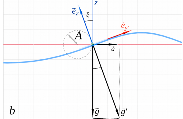
F i g.  1. Sketch explaining the accepted notation and the principle of inertial measurement of waves in the x'y'z' frame moving with liquid particles: general view (a), side view along the x-axis (b). The wave propagates in the positive direction of the x-axis of the right fixed reference frame

Therefore, an estimate of the wave height can be obtained by double integration of the measured accelerations, or, equivalently, in the spectral domain, by relating the spectra of the heights and accelerations. Therefore,

Szω=ω-4Saω,                                               (2)

where Sz  is the elevation spectrum, Sa  is the acceleration spectrum, ω=2πf is the radial frequency representing the Fourier frequency domain (not the single harmonic Ω ). Similar estimates can also be written for slope spectra (or magnetic measurements) Sξ and rotation rate spectra (or gyroscope measurements) Sη , taking into account the linear dispersion relation:

Szω=g2ω-4Sξω,

Szω=g2ω-6Sηω.                                        (3)

All three estimates have a singularity, Sz→∞  for ω→0,  which distorts the integral estimates such as SWH, Hs=4Szωdω.  To avoid uncertainty, the low-frequency oscillations are usually suppressed by a high-pass filter. The characteristic frequency of this filter must be explicitly specified, e.g., empirically based on the typical or minimum possible frequency observed in a given water body, or can be a tuning parameter of the filter that separates signal from noise [13, 30–32].

Equipment. In this work, conventional commercial off-the-shelf IMUs were used. Table lists some parameters of the most accessible models on the market, including Russian devices. Based on the chip package size and typical parameters of the measured waves, the applicability of these modules for wave measurements can be assessed.

In particular, the magnitude of the liquid particle wave acceleration, a=AΩ2==AKg , is usually smaller than the acceleration of gravity, because waves break when AK>0.44…0.55  [33]. Therefore, it is optimal to select the acceleration measurement range within (1…2)g , both for the most efficient use of the analog-to-digital converter dynamic range and for possible wave breaking moments filtering and/or analysis.

Unlike acceleration, the rotation rate measured by a gyroscope depends not only on the steepness of the wave, but also on its frequency, η=AKΩ.  The maximum recorded frequency, which has a practical meaning, is determined by the geometry of the buoy hull, i.e., the frequencies of the resonant oscillations and the cut-off frequency of the hull. For example, for the Datawell [34] and Spotter [22] buoys, both 40 cm in diameter, this frequency is set to 0.6 Hz and 1 Hz, respectively. These frequencies correspond to ~ 120 and ~ 200 º/s rotation rates, falling within the first two ranges that can be selected with most sensors.

Magnetometer measurements in wave sensing applications are usually limited to recording the geomagnetic field with typical values of (25...65) µT, which is a standard task for most sensors.

Thus, the measurement ranges of the simplest (cheapest) sensors provide the means to confidently use them for wave measurements. It should also be noted that the bandwidths of the accelerometer and gyroscope are in the order of tens to hundreds of Hz (nominally for vibration measurements). This is particularly important for shortest wave measurements [29] and wind speed estimates [35]. The nonlinearity and calibration coefficient errors are typically less than 1%, a very good relative error for in situ wave height measurements. Many IMUs (e.g. BNO-055 and MG-10 in Table) are equipped with a built-in algorithm for processing inertial measurements. However, such algorithms are usually not documented, and the only tuning parameter available to the user is the sensor sampling frequency. Therefore, it is preferable to implement a specialized data processing algorithm that takes into account the characteristics inherent in sea wave motion.

Characteristics of some commercial IMUs

* The range can be adjusted upon request.

A critical parameter for wave measuring is the intrinsic noise of the sensors. In fact, according to (2–4), spectral estimates at low-frequencies are artificially “amplified” by multiplying the spectrum by a rather high negative frequency power (−4 or −6) – in the spectral domain – or by integrating it twice or thrice – in the time domain. Obviously, the presence of broadband inherent noise can lead to critical errors in the estimation of wave parameters, as will be discussed below.

In general, the sensors listed in Table have noise characteristics that are similar in magnitude. The MPU-9250 sensor, which combines an accelerometer/gyroscope/magnetometer, was chosen as a sample for more detailed testing. On the one hand, this is the most affordable model on the Russian market at the time of the study. On the other hand, a sensor of this model was already available to us as part of a wave buoy prototype that has been operating episodically for five years [20, 29]. This helps to evaluate the effects of MEMS aging for this model. In addition to this sample, five similar IMUs from different production series were used in the tests.

The intrinsic noise characteristics were evaluated in static mode (the sensor is stationary) at various ambient temperatures ranging from −10 to 50 ºС.

IMU data processing. The sea surface elevation spectra were calculated from the vertical accelerations according to the formula (2). Vertical accelerations in the fixed reference frame can be estimated from inertial data in different ways. Four algorithms based on different approaches are considered.

Algorithm А1. It is assumed that the vertical acceleration variations of the sensor in the fixed reference frame coincide with the vertical acceleration variations measured in the moving reference frame according to the formula (1). This assumption is valid for the buoy perfectly following the wave slopes, which must be small (no resonance oscillations of the buoy, waves are linear).

Algorithm А2/А3. The vertical accelerations of liquid particles can also be obtained by knowing the instantaneous orientation of the moving reference frame. The orientation of one reference frame relative to another can be uniquely determined if the coordinates of two non-collinear vectors in each of these systems are known. Based on this statement, the so-called TRIAD method was developed [14, 15]. If p  and q are the vector pair in the xyz reference frame, while p'  and q' are the  corresponding vector pair in the x'y'z' reference frame, then the rotation matrix between xyz and x'y'z' can be written as R=r1 r2 r3⋅s1 s2 s3T,  where r1 r2 r3  and s1 s2 s3  are the matrices obtained by the horizontal concatenation of the following vector triads: r1=p' , r2=p'×q' ,  r3=r1×r2  , and s1=p ,   s2==p×q ,  s3=s1×s2 .

For standard inertial measurements, only two vectors can be used as a reference: the acceleration of gravity, g , and the geomagnetic field, m . The TRIAD method provides an exact solution only in the case of uniform rectilinear motion. In the case of accelerated motion, i.e., wave orbital motion, the measured acceleration does not coincide with the gravity force in the moving reference frame. Therefore, the TRIAD method requires the sensor accelerations to be much smaller than the acceleration of gravity, a≪g  , or AK≪1 , the same condition as for the A1 algorithm. However, unlike А1, the resonant buoy oscillations can be accounted for. 

The TRIAD transform is invariant with respect to the permutation of p  and q  only if the angle between them is constant. Otherwise, if ∠p,q-∠p',q'=ε , the estimated rotation transform R exactly matches only p  and p' , but not q and q' ,  i.e., ∠p,p'⋅R=0 and ∠q,q'⋅R=ε. Thus, for accelerated (wave) motion, the order of the reference vectors is important: p=g , q=m  or p=m , q=g .  Depending on this choice, the priority vector, p , will be either the acceleration vector or the magnetic field vector. In our notations, the A2 algorithm corresponds to
p=g (gravity priority), while the A3 algorithm corresponds to p=m (magnetic field priority).

Algorithm А4 is based on the Kalman filter, which assimilates all three types of inertial data [16, 17]. We use the open-source implementation of this algorithm, which is documented in (https://github.com/memsindustrygroup/Open-Source-Sensor-Fusion). Unlike the А2/А3 algorithms, which provide the orientation directly, the Kalman filter recursively assimilates the estimation errors of the acceleration, rotation rates and magnetic field, and improves the current estimate of the orientation based on the error model. Note that such a filtering is used in the most advanced IMU-based wave buoys [18, 21, 24, 25, 36].

Field data were obtained in an experiment from the Stationary Oceanographic Platform of Marine Hydrophysical Institute using a wave buoy prototype (float diameter is 15 cm) built on the basis of the MPU-9250 sensor [29]. Simultaneously with the buoy measurements, vertical elevations of the sea surface were recorded by a six-channel resistive wave gauge at a distance of 100–150 m from the buoy [37, 38]. The accuracy of the wave gauge measurement is 1 cm in the 0.1–5 Hz frequency band (sampling frequency is 10 Hz).

Two time series of 30 min each, obtained under different wind and wave conditions, are used. The first case corresponds to a developing sea: wind speed was 13.1 m/s; SWH was 0.7 m; the spectrum measured by the wave gauge had a peak at 0.25 Hz (inverse wave age is 2.1). In the second case, a mixed sea was observed: wind speed was 5.2 m/s; SWH was 0.2 m; the spectrum had two peaks, one corresponding to the wind waves at a frequency of 0.5 Hz and the second swell peak at a frequency of 0.15–0.2 Hz.

Results and discussion

Sensor static noise. The noise characteristics for the selected IMU samples are shown in Fig. 2. The standard deviation (STD) of the accelerometer static noise signals depends almost linearly on the sensor temperature, with the z-component noise being 1.5–2 times higher than the x- and y-component noise. At the same time, even the maximum observed value of ~ 2 mg is approximately 4 times lower than the STD value of 8 mg declared in the sensor specification. A similar trend is observed for the spectral noise density measured at a sensor temperature of (20 ± 2) °C (Fig. 2, b). At frequencies above 0.1 Hz, the noise spectrum level for the z-component is higher, but not higher than the specification value (shown by the dotted line).

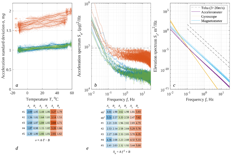
F i g.  2. Measured intrinsic noise of accelerometer channels for the MPU-9250 inertial motion unit: the acceleration standard deviation versus temperature (a), acceleration noise spectrum (b), equivalent elevation spectra estimated from accelerometer, gyroscope, and magnetometer data (c); heat map of fitting coefficients for the curves shown in panel a (A – in [μg/°C], B – in [mg]) (d); heat map of fitting coefficients for the curves shown in panel b (A – in [(μg)² · 10⁻³], B – in [(μg)²/Hz · 10⁻⁴]) (e)

At frequencies below 0.1 Hz, the noise spectrum becomes higher than the specification level and has a 1/f slope indicating its non-thermal nature (flicker noise [39]). Sample #0, used periodically for five years (curves #0¹ and #0²), shows an increase in spectral noise density by a factor of ~ 1.3, but this value does not exceed the specification values.

The similar behavior, a good agreement with the specification levels, is also observed for the noise of the gyroscope and magnetometer channels, which are not shown in the figures for brevity. Instead, Fig. 2, c shows the equivalent elevation spectra estimated from (2–4) for all three types of inertial measurements. As can be seen from the Figure, the most noise is expected in the spectra obtained from the magnetometer channel (blue lines). With the same f-4  slope, these spectra are ~ 1–1.5 orders of magnitude higher than the corresponding noise spectra estimated from accelerometer measurements (purple lines). The noise spectra estimated from rotation rates (yellow lines), in accordance with the formula (3), have a f-6  slope, resulting in a much higher spectral noise density at frequencies below 0.1 Hz. Note, however, that the expected elevation spectra for the real sea surface (the Toba spectrum [40] at 3–20 m/s wind speed shown for reference in Fig. 2, c by dashed lines) are 4–5 orders of magnitude higher than any equivalent noise spectra. Thus, the intrinsic noise of the sensors can be neglected when estimating the real wind wave elevation spectra.

Field measurements. To estimate the elevation spectra from in situ data, the А1–А4 algorithms were applied to the raw accelerometer/gyroscope/ /magnetometer records. An example of such processing for typical conditions (developing sea, wind speed is 13.1 m/s) is shown in Fig. 3, which demonstrates a fragment of the vertical acceleration record in a moving reference frame (A1) in comparison with the results of processing by the TRIAD method (A2/A3) and the Kalman filter (A4).

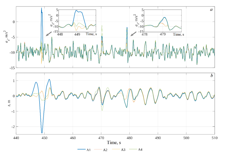
F i g.  3. Vertical acceleration time series (a) and vertical displacement after 5 s high-pass filtering (b) estimated using algorithms A1–A4. The subpanels show the wave breaking events at 449 s and 479 s  in more detail

In general, the corrections introduced by the A2–A4 algorithms are not large, indicating the smallness of the slopes. The exception is the case of sharp spikes associated with wave breaking. In Fig. 3, a fragment with three such events (at 448 s, 470 s, 478 s) occurring within 30 s was deliberately selected. The TRIAD method (A2/A3) smooths such spikes, whereas the use of the Kalman filter (A4) can lead to an increase of the burst (events at 470 s, 478 s). We also note the presence of a certain relaxation time for the A4 algorithm, which is required to readjust the Kalman filter after a sharp jump in all measured parameters (interval 450–470 s).

The sea surface elevations obtained by integrating the accelerations are shown in Fig. 3, b. The low-frequency components of the accelerations introduce unacceptable errors into this signal, so for this Figure the original series are high-pass filtered with a time constant equal to the period of the peak waves, 5 s. During the event at 449 s, the height difference according to algorithm A1 is unrealistically large, more than 3 m, while the SWH is about 0.7 m. The reason is obviously the penetration of horizontal accelerations into the vertical acceleration signal due to the fact that the hull orientation is not taken into account by the A1 algorithm. The corrections introduced by the A2–A4 algorithms allow the smoothing of such spikes, as can be seen in Fig. 3, b

Figure 4 a, c shows the elevation spectra calculated from 30-min records under developing and mixed sea conditions, with the initial time series divided into successive 1-min intervals and further averaging over them. These estimates are based on vertical accelerations obtained using the A1–A4 algorithms (colored lines). The elevation spectra measured by the wave gauge (black lines) are given as a reference. In the operating frequency range (0.2–1 Hz), all spectral estimates agree within the confidence intervals, as well as with the empirical level of the Toba spectrum [40], regardless of the choice of the processing algorithm. At frequencies above 1 Hz, the possible deviations are related to the transfer function of the buoy hull and to Doppler distortions of the reference wave gauge spectra [41].

The main differences between the algorithms are observed at frequencies below the peak frequency f_p. For the case of the developing sea (Fig. 4, a), the contrast of the spectral peak to the low frequency noise background is ~ 7 for the moving frame vertical accelerations (A1), ~ 16 for the TRIAD method (A2/A3), and ~ 1.5 for the Kalman filter (A4). Hereinafter, the “low-frequency” corresponds to the oscillations with frequencies below the peak frequency, 0 < f < f_p. In the case of the mixed sea (Fig. 4, c), a similar tendency remains, but the contrast is several times smaller, about 2–4.

The low frequency noise is critically important when estimating the SWH. The elevation spectrum decreases rather rapidly with frequency (f-4 ), so that the main contribution to the SWH comes from the longest waves, which, as follows from the results presented, are measured quite well up to the spectral peak. However, the presence of low frequency noise below the peak requires the correct choice of the lower integration limit when estimating the SWH. This statement is illustrated in Figure 4 b, d, which shows the cumulative values of SWH depending on the lower integration limit (plotted along the horizontal frequency axis):

Hsf=4Sf'df' .

For instance, if the lower limit is 0, then the SWH (left axis in Fig. 4 b, d) and its relative error 1-HsfpHs  (right axis in the same plot) tend to infinity (the colored lines bend upwards at f→0 ), see (2).

If the lower limit is equal to the frequency of the first inflection of the spectrum to the left of the spectral peak (shown by vertical dashed dotted lines), the relative measurement error will not exceed 2% for A2/A3 algorithms and 10% for A1, A4 algorithms. However, this method of searching for the lower integration boundary has its limitations, since a swell signal can also be observed below f_p. For example, if the wind peak in the situation shown in Fig. 4, c was higher than the swell peak.

An alternative signal/noise boundary can be a frequency identified by the first (from the f=0  side) minimum in the spectrum. These points for all four algorithms are shown as encircled crosses in Fig. 4. In the case of such an automated search, the relative SWH error also lies within 10%. However, this method is not always efficient, since the first local minimum can be at a significantly lower frequency due to the random nature of the wave signal, while the errors become unacceptable at f→0  due to the f-4 -slope of the spectrum.

The issue of filtering low-frequency noise is traditional for buoy data processing. For example, it has been proposed to use a priori information about the shape of the spectrum [30, 42], the ratio of the amplitudes of vertical and horizontal motions [10], and various empirical corrections [11, 13]. However, the origin of the low-frequency noise does not seem to be related to the internal characteristics of the sensor, because, firstly, the measured intrinsic noise is 3–4 orders weaker, as follows from the comparison of Fig. 4 and Fig. 2, and, secondly, it depends significantly on the signal processing method (Fig. 4). Therefore, the origin of this noise requires additional discussion.

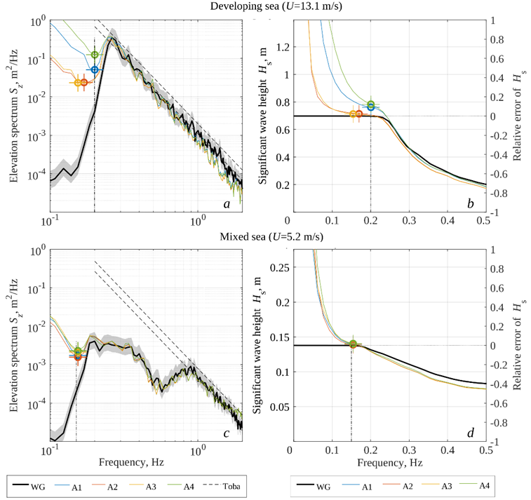
F i g.  4. Sea surface elevation spectra (a, c) and significant wave height relative error (b, d) measured in the field experiment. The colored lines show the results of the processing by the A1–A4 algorithms, the thick black line shows the reference measurements by wire wave gauge. Symbols (+) indicate the first local minimum in the spectrum. The vertical dash-dotted line shows the frequency corresponding to the inflection point in the spectrum

Numerical simulation. The following numerical simulation was performed to illustrate the features of the data processing algorithms. The initial unperturbed sea surface, defined as a flat uniform grid, is deformed by a superposition of N Gerstner waves,

Xm=RealAmnsinθn,

Ym=RealAmncosθn,

Zm=ImagAmn,

Amn=2⋅Sfn⋅ΔfN⋅expiKxn⋅xm+Kyn⋅ym-2πfnt+ϕn,

where Sfn  is the Toba spectrum, Δf=fN-f1  is the frequency band in which the simulation is performed, the frequency limits are f1=0.2  Hz, fN=4  Hz, ϕn  is the random phase uniformly distributed within 0,2π , θn  is the random wave direction normally distributed around zero mean (waves travel along the y-axis). The complex amplitude, A_mn, reproduces the target spectrum  Sfn  for which the Toba spectrum is adopted again. The angular width is set to 45º in accordance with typical values of this parameter for the real sea surface [43]. The grid size is δx=δy=0.01  m, the time step is δt=0.1 s, the simulation domain is Δx=Δy=2  m, the simulation duration is Δt=1800  s, the number of harmonics is N=Δf⋅Δt . The magnetic field is directed along the x- or y-axis, depending on the simulation run.

Despite some issues regarding the feasibility of Gerstner waves on the real sea surface [44], this approach has become widespread due to the possibility of taking into account the nonlinearity of waves [45–47]. In the present study, it is particularly convenient because it allows to simulate the motion of liquid particles, and thus the motion of a free-floating body “attached” to them, without numerically solving the hydrodynamic equations. In particular, it is assumed that a flat round buoy (15 cm in diameter, as in the field experiment) equipped with an IMU “lies” on the simulated surface without experiencing its own resonant oscillations (the buoy thickness is zero). The position of such a virtual buoy is determined at each moment by fitting the liquid particles under the buoy with a plane. Based on the known positions of the buoy center and its orientations, the inertial sensor measurements are simulated, i.e., accelerations, rotation rates, and magnetic field components in a moving reference frame.

With this simulation data set, it is possible to check how adequately the inverse problem of estimating wave parameters from inertial measurements is solved by one or another algorithm. Figure 5 shows an example of a simulation for a five-second interval, corresponding to one period of peak waves. The buoy orientation is shown by colored arrows in different scales: the long arrows are the true (estimated) orientation, the medium-length arrows show the TRIAD method estimate, the short arrows are the Kalman filter estimates (A4). Note that the A1 algorithm does not include an orientation estimate.

As can be seen from this example, all the considered methods provide generally reliable orientation in the direction of the x-axis (red unit vectors). This is explained by the small variability of the slope in this direction, since the waves in this simulation propagate along the y-axis. Accordingly, the main differences from the true values are observed in the yz-plane (blue and green unit vectors). The errors of the Kalman filter algorithm (A4) are generally smaller than those of the TRIAD method. But for the latter, the choice of the priority vector is crucial. If the magnetic field is chosen (in this example it is aligned with the direction of the waves), then the orientation retrieval is perfect. If the gravity vector is chosen, then the errors are larger than for the Kalman filter.

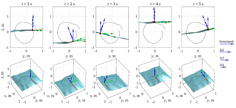
F i g.  5. An example showing a numerical simulation of the sea surface during a peak wave period for five equally spaced instants: side view – on the top, general view – on the bottom. The colored arrows show the orientations of the virtual buoy estimated by algorithms A2–A4, the black line is the trajectory of the buoy

These features are illustrated in more detail in Fig. 6, where the instantaneous orientations are shown as Euler angle time series, roll/pitch/azimuth, where roll is the slope angle along the y-axis, pitch is the slope angle along the x-axis, and azimuth angle is the rotation around the z-axis. In particular, pitch and azimuth are reproduced equally poorly by the TRIAD method (the curves A2 and A3 completely coincide), while true roll (blue thick line) is reproduced perfectly by the A3 algorithm (the red curve completely coincides with the blue thick line), contrary to the A2 algorithm. Thus, the main disadvantage of the TRIAD method is its sensitivity to the direction of the waves relative to the magnetic field vector, as well as to the choice of the priority vector (gravity or acceleration).

As with the Kalman filter, the roll and pitch are reproduced with approximately the same accuracy, but with a small delay relative to the true signal. Of critical importance to this study is the “stray” noise, which is clearly visible in the azimuth signal in Fig. 6. The true value of the azimuth angle is virtually constant, while the A4 curve randomly deviates from the mean value within ±10º, and, most importantly, with a period exceeding the period of the wave peak. Note also that the same low frequency oscillations are present, although less distinguishable, in the roll and pitch angles.  For example, the A4 curve (green) is slightly higher than the true curve (blue) before ~ 13 s of the simulation, but later it becomes lower. At first glance, such a small error < 5º may seem insignificant. However, it can be a strong artifact in the elevation spectra, as shown below in the same way as for the field data analysis.

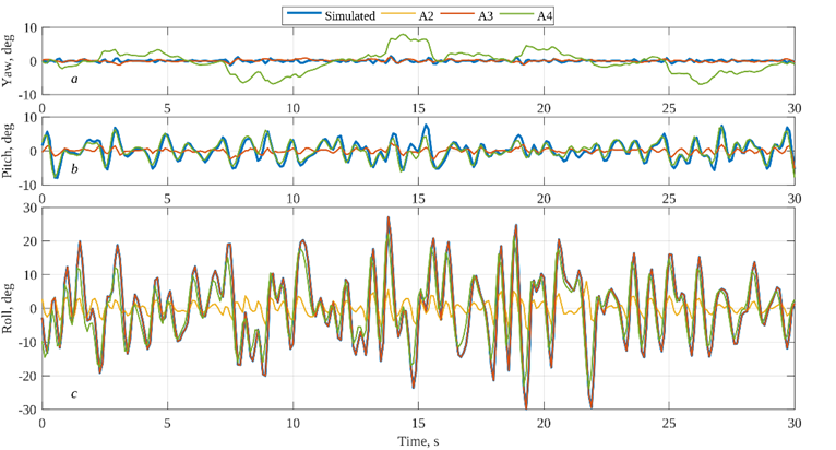
F i g.  6. Euler angles (roll/pitch/yaw) estimated using algorithms A2–A4 based on model calculations

Three different wave situations with peak frequencies fp=  0.3, 0.2, 0.1 Hz are considered in Fig. 7 (left, middle and right columns, respectively). The wind speed, which determines the spectral level in the target Toba spectrum, is chosen to be equal to U = 5.2, 7.8, 15.6 m/s, respectively, based on the condition for the wave age cpU=1 , where U is the wind speed, сp=g2πfp  is the phase velocity of the spectral peak waves. For these three situations, two cases are analyzed, the waves are co-aligned with the magnetic field (top row in Fig. 7) and perpendicular to the magnetic field (bottom row).

Comparing the simulation results with the field measurements (Fig. 7 and Fig. 4), one can note their close similarity. Despite the rather primitive simulation scheme (no resonant hull oscillations, perfect wave following, representation of the surface by a set of Gerstner waves), the numerical simulations exhibit the same characteristics as for the real sea. Particularly, an almost complete agreement of the estimates with the true value in the operating frequency range fp<f<1  Hz; a “fall-off” of the spectral density in the higher frequency range in accordance with the transfer function of the hull; the presence of low frequency noise. Regarding the latter, the level of low frequency noise may differ by a factor of 3–4, depending on the choice of data processing algorithm.

The strongest low frequency noise is introduced by the Kalman filter (A4). For example, at the wind speeds above 15 m/s, the spectral peak becomes barely distinguishable (Fig. 7, f) or indistinguishable (Fig. 7, c) depending on the direction of the waves relative to the magnetic field. The dependence on the wave azimuth is much greater for algorithms based on the TRIAD method (A2/A3). The worst performance is obtained with the A3 algorithm (magnetic field priority) when the orientation of the waves and the magnetic field are perpendicular to each other. The A2 algorithm (gravity priority) produces a level of low frequency noise comparable to the A1 algorithm, which assumes that the buoy perfectly follows the wave slopes (the default option in these simulations).

Thus, the conducted numerical simulation clearly demonstrates that the level of the intrinsic noise of modern inertial sensors (e.g., the noise of the MPU-9250 sensor is shown by the blue lines in Fig. 7) is negligibly small, compared to both the wave signal and the low frequency noise. The latter, based on the problem formulation, can only be generated by the nonlinearity in the response of the measuring device to wave surface. Particularly, the average slope and elevation of the buoy in this simulation is based on always changing ensembles of liquid particles.

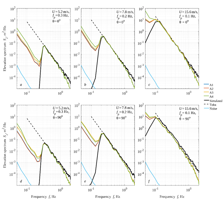
F i g.  7. Elevation spectra estimated from virtual buoy measurements (colored lines) compared to the true spectrum (thick black line). The direction of the waves in the numerical experiment is along the magnetic field – on the top, across the magnetic field – on the bottom. The peak wave frequency is 0.3 Hz (on the left), 0.2 Hz (in the middle), 0.1 Hz (on the right) with a constant wave age equal to 1

Similar non-linear effects are manifested as low frequency noise in various dynamic systems, such as infra-gravity waves [48], acoustic noise of the sea [49], etc. In the considered sea surface-buoy system, the nonlinearity is inherent both in the surface itself and in the estimation of the surface slope. In the case of the Kalman filter, the recursive transform is ambiguous, i.e., the estimate in the current step depends on the result of the calculation in the previous step.

It should also be noted that in the real conditions there are usually many more sources of noise. These include the hull resonance oscillations, which are generally non-linear because the dependence of the buoyancy force and the restoring moment on the current draft and tilt of the buoy is determined by the shape of the hull and the mass distribution within it. The holding line response (if present) can also be important [11], as can biofouling [50] and the interaction of the buoy hull with wind [51] and currents [52]. Obviously, all these factors may impact the measurement errors. At the same time, the technical characteristics of modern inertial sensors play a minor role, as can be seen from the present results.

Conclusion

This paper presents the results of laboratory, field, and numerical experiments to assess the applicability of the modern conventional MEMS inertial motion units (IMUs) in wave buoys. The main conclusions are as follows:

– various methods of estimating wave heights based on measurements from standard IMUs (accelerometer/gyroscope/magnetometer) are considered. The most suitable method is based on the analysis of the vertical accelerations of the sensor in a fixed reference frame. Four algorithms are considered for estimating vertical accelerations, based on (a) the assumption of perfect wave following, (b) the so-called TRIAD method, which is an exact solution only for uniform motion, and (c) the recursive Kalman filter, which is the most popular solution in navigation problems;

– laboratory tests have shown that the static accelerometer noise of a typical IMU is 3-4 orders of magnitude lower than the surface wave signal, and the accuracy characteristics of such sensors ensure that wave heights are measured with an error not exceeding the specification values, which is typically no more than 3%. The error in estimated wave height from the field wave buoy measurements is within 2% in the spectral peak band ranging from 0.2 to 0.25 Hz;

– the noise at frequencies below the spectral peak can be a serious problem for wave height estimation as it prevents the wave signal from being confidently distinguished. For example, the error in estimating the significant wave height increases to 10% when the spectrum is integrated from the signal/noise separating frequency estimated from the first local minimum condition. The error can become unacceptable when a low frequency spectral peak is mistakenly detected due to the “gain factor” f-4  that relates the acceleration and elevation spectra;

– in order to determine the origin of the low frequency noise, a numerical experiment was performed to simulate the signals of an idealized IMU-based buoy and to retrieve the wave parameters from them. A sufficient condition for the occurrence of such noise is the nonlinearity of the sea surface, which is present in the simulated superposition of Gerstner waves. Even without taking into account the resonant oscillations of the hull (a zero-thickness buoy), the results of the numerical experiment reproduce almost all the details of the field measurements, including the low frequency noise;

– the highest level of low frequency noise, both in the field and in the numerical experiments, is observed when the Kalman filter is used to determine the buoy current orientation. Thus, the minimization of the wave height measurement error is more sensitive to the choice of the data processing algorithm than to the choice of a specific sensor model.

1. Earle, M.D. and Bishop, J.M., 1984. A Practical Guide to Ocean Wave Measurement and Analysis. Marion, MA, USA: Endeco Inc., 78 p.

2. McCall, J.C., 1998. Advances in National Data Buoy Center Technology. In: IEEE Oceanic Engineering Society, 1998. OCEANS’98. Conference Proceedings (Cat. No. 98CH36259). Nice, France: IEEE. Vol. 1, pp. 544-548. https://doi.org/10.1109/OCEANS.1998.72806

3. Lobanov, V.B., Lazaryuk, A.Yu., Ponomarev, V.I., Sergeev, A.F., Marina, E.N., Starjinskii, S.S., Kharlamov, P.O., Shkorba, S.P. [et al.], 2020. The Results of Hydrometeorological Measurements by the WAVESCAN Buoy System on the Southwestern Shelf of the Peter the Great Bay in 2016. Journal of Oceanological Research, 48(4), pp. 5-31. https://doi.org/10.29006/1564-2291.JOR-2020.48(4).1

4. Divinsky, B.V. and Kuklev, S.B., 2022. Experiment of Wind Wave Parameter Research in the Black Sea Shelf. Oceanology, 62(1), pp. 8-12. https://doi.org/10.1134/S0001437022010040

5. Longuet-Higgins, M.S., Cartwright, D.E. and Smith, N.D., 1963. Observations of the Directional Spectrum of Sea Waves Using the Motions of a Floating Buoy. In: National Academy of Sciences, 1963. Ocean Wave Spectra: Proceedings of a Conference. Prentice-Hall, Englewood Cliffs, N.J., pp. 111-132.

6. Gryazin, D. and Gleb, K., 2022. A New Method to Determine Directional Spectrum of Sea Waves and Its Application to Wave Buoys. Journal of Ocean Engineering and Marine Energy, 8(3), pp. 269-283. https://doi.org/10.1007/s40722-022-00228-z

7. Herbers, T.H.C., Jessen, P.F., Janssen, T.T., Colbert, D.B. and MacMahan, J.H., 2012. Observing Ocean Surface Waves with GPS-Tracked Buoys. Journal of Atmospheric and Oceanic Technology, 29(7), pp. 944-959. https://doi.org/10.1175/JTECH-D-11-00128.1

8. Shimura, T., Mori, N., Baba, Y. and Miyashita, T., 2022. Ocean Surface Wind Estimation from Waves Based on Small GPS Buoy Observations in a Bay and the Open Ocean. Journal of Geophysical Research: Oceans, 127(9), e2022JC018786. https://doi.org/10.1029/2022JC018786

9. Collins, C.O., Dickhudt, P., Thompson, J., de Paolo, T., Otero, M., Merrifield, S., Terrill, E., Schonau, M., Braasch, L. [et al.], 2024. Performance of Moored GPS Wave Buoys. Coastal Engineering Journal, 66(1), pp. 17-43. https://doi.org/10.1080/21664250.2023.2295105

10. Stewart, R.H., 1977. A Discus-Hulled Wave Measuring Buoy. Ocean Engineering, 4(2), pp. 101-107.

11. Earle, M.D., 1996. Nondirectional and Directional Wave Data Analysis Procedures. NDBC Technical Document 96-01. Slidell, USA: Stennis Space Center, 43 p.

12. Earle, M. and Bush, K., 1982. Strapped-Down Accelerometer Effects on NDBO Wave Measurements. In: Marine Technology Society, IEEE, 1982. OCEANS 82 Conference Record. Washington, DC, USA, pp. 838-848. https://doi.org/10.1109/OCEANS.1982.1151908

13. Earle, M., Steele, K. and Hsu, Y.-H., 1984. Wave Spectra Corrections for Measurements of Hull-Fixed Accelerometers. In: Marine Technology Society, IEEE, 1984. OCEANS 84 Conference Record. Washington, DC, USA, pp. 725-730. https://doi.org/10.1109/OCEANS.1984.1152234

14. Black, H.D., 1964. A Passive System for Determining the Attitude of a Satellite. AIAA Journal, 2(7), pp. 1350-1351. https://doi.org/10.2514/3.2555

15. Shuster, M.D. and Oh, S.D., 1981. Three-Axis Attitude Determination from Vector Observations. Journal of Guidance and Control, 4(1), pp. 70-77. https://doi.org/10.2514/3.19717

16. Sabatini, A.M., 2011. Kalman-Filter-Based Orientation Determination Using Inertial/Magnetic Sensors: Observability Analysis and Performance Evaluation. Sensors, 11(10), pp. 9182-9206. https://doi.org/10.3390/s111009182

17. Wang, L., Zhang, Z. and Sun, P., 2015. Quaternion-Based Kalman Filter for AHRS Using an Adaptive-Step Gradient Descent Algorithm. International Journal of Advanced Robotic Systems, 12(9), 131. https://doi.org/10.5772/61313

18. Rabault, J., Nose, T., Hope, G., Muller, M., Breivik, O., Voermans, J., Hole, L.R., Bohlinger, P., Waseda, T. [et al.], 2022. OpenMetBuoy-v2021: An Easy-to-Build, Affordable, Customizable, Open Source Instrument for Oceanographic Measurements of Drift and Waves in Sea Ice and the Open Ocean. Geosciences, 12(3), 110. https://doi.org/10.13140/RG.2.2.15826.07368

19. MacIsaac, C. and Naeth, S., 2013. TRIAXYS Next Wave II Directional Wave Sensor the Evolution of Wave Measurements. In: IEEE, 2013. OCEANS 2013. San Diego, California, USA, pp. 2002-2010.

20. Yurovsky, Y.Y. and Dulov, V.A., 2017. Compact Low-Cost Arduino-Based Buoy for Sea Surface Wave Measurements. In: IEEE, 2017. 2017 Progress in Electromagnetics Research Symposium – Fall (PIERS – FALL). Singapore, pp. 2315-2322. https://doi.org/10.1109/PIERS-FALL.2017.8293523

21. Veras Guimarães, P., Ardhuin, F., Sutherland, P., Accensi, M., Hamon, M., Pérignon, Y., Thompson, J., Benetazzo, A. and Ferrant, P., 2018. A Surface Kinematics Buoy (SKIB) for Wave–Current Interaction Studies. Ocean Science, 14(6), pp. 1449-1460. https://doi.org/10.5194/os-14-1449-2018

22. Raghukumar, K., Chang, G., Spada, F., Jones, C., Janssen, T. and Gans, A., 2019. Performance Characteristics of “Spotter,” a Newly Developed Real-Time Wave Measurement Buoy. Journal of Atmospheric and Oceanic Technology, 36(6), pp. 1127-1141. https://doi.org/10.1175/JTECH-D-18-0151.1

23. Houghton, I.A., Smit, P.B., Clark, D., Dunning, C., Fisher, A., Nidzieko, N.J., Chamberlain, P. and Janssen, T.T., 2021. Performance Statistics of a Real-Time Pacific Ocean Weather Sensor Network. Journal of Atmospheric and Oceanic Technology, 38(5), pp. 1047-1058. https://doi.org/10.1175/JTECH-D-20-0187.1

24. Rainville, E., Thompson, J., Moulton, M. and Derakhti, M., 2023. Measurements of Nearshore Ocean-Surface Kinematics through Coherent Arrays of Free-Drifting Buoys. Earth System Science Data, 15(11), pp. 5135-5151. https://doi.org/10.5194/essd-15-5135-2023

25. Zhong, Y.-Z., Chien, H., Chang, H.-M. and Cheng, H.-Y., 2022. Ocean Wind Observation Based on the Mean Square Slope Using a Self-Developed Miniature Wave Buoy. Sensors, 22(19), 7210. https://doi.org/10.3390/s22197210

26. Alari, V., Björkqvist, J.-V., Kaldvee, V., Mölder, K., Rikka, S., Kask-Korb, A., Vahter, K., Pärt, S., Vidjajev, N. [et al.], 2022. LainePoiss® – A Lightweight and Ice-Resistant Wave Buoy. Journal of Atmospheric and Oceanic Technology, 39(5), pp. 573-594. https://doi.org/10.1175/JTECH-D-21-0091.1

27. Mironov, A.S. and Charron, L., 2023. Miniaturized Drifting Buoy Platform for the Creation of Undersatellite Calibration and Validation Network. In: IEEE, 2023. OCEANS 2023 – Limerick. Limerick, Ireland: IEEE, pp. 1-10.

28. Thomson, J., Bush, P., Contreras, V.C., Clemett, N., Davis, J., de Klerk, A., Iseley, E. and Rainville, E.J., 2024. Development and Testing of MicroSWIFT Expendable Wave Buoys. Coastal Engineering Journal, 66(1), pp. 168-180. https://doi.org/10.1080/21664250.2023.2283325

29. Yurovsky, Y.Yu. and Dulov, V.A., 2020. MEMS-Based Wave Buoy: Towards Short Wind-Wave Sensing. Ocean Engineering, 217, 108043. https://doi.org/10.1016/j.oceaneng.2020.108043

30. Ashton, I.G.C. and Johanning, L., 2015. On Errors in Low Frequency Wave Measurements from Wave Buoys. Ocean Engineering, 95, pp. 11-22. https://doi.org/10.1016/j.oceaneng.2014.11.033

31. Ding, Y., Taylor, P.H., Zhao, W., Dory, J.-N., Hlophe, T. and Draper, S., 2023. Oceanographic Wave Buoy Motion as a 3D-Vector Field: Spectra, Linear Components and Bound Harmonics. Applied Ocean Research, 141, 103777. https://doi.org/10.1016/j.apor.2023.103777

32. Amarouche, K., Akpinar, A., Rybalko, A. and Myslenkov, S., 2023. Assessment of SWAN and WAVEWATCH-III Models Regarding the Directional Wave Spectra Estimates Based on Eastern Black Sea Measurements. Ocean Engineering, 272, 113944. https://doi.org/10.1016/j.oceaneng.2023.113944

33. Toffoli, A., Babanin, A., Onorato, M. and Waseda, T., 2010. Maximum Steepness of Oceanic Waves: Field and Laboratory Experiments. Geophysical Research Letters, 37(5), L05603. https://doi.org/10.1029/2009GL041771

34. Jeans, G., Bellamy, I., de Vries, J.J. and van Weert, P., 2003. Sea Trial of the New Datawell GPS Directional Waverider. In: J. A. Rizoli, ed., 2003. Proceedings of the IEEE-OES Seventh Working Conference on Current Measurement Technology. San Diego, CA, USA, pp. 145-147. https://doi.org/10.1109/CCM.2003.1194302

35. Rybalko, A., Myslenkov, S. and Badulin, S., 2023. Wave Buoy Measurements at Short Fetches in the Black Sea Nearshore: Mixed Sea and Energy Fluxes. Water, 15(10), 1834. https://doi.org/10.3390/w15101834

36. Kodaira, T., Katsuno, T., Nose, T., Itoh, M., Rabault, J., Hoppmann, M., Kimizuka, M. and Waseda, T., 2023. An Affordable and Customizable Wave Buoy for the Study of Wave-Ice Interactions: Design Concept and Results from Field Deployments. Coastal Engineering Journal, 66(1), pp. 74-88. https://doi.org/10.1080/21664250.2023.2249243

37. Bondur, V.G., Dulov, V.A., Murynin, A.B. and Yurovsky, Yu.Yu., 2016. A Study of Sea-Wave Spectra in a Wide Wavelength Range from Satellite and In-Situ Data. Izvestiya, Atmospheric and Oceanic Physics, 52(9), pp. 888-903. https://doi.org/10.1134/S0001433816090097

38. Smolov, V.E. and Rozvadovskiy, A.F., 2020. Application of the Arduino Platform for Recording Wind Waves. Physical Oceanography, 27(4), pp. 430-441. https://doi.org/10.22449/1573-160X-2020-4-430-441

39. Mohd-Yasin, F., Korman, C.E. and Nagel, D.J., 2003. Measurement of Noise Characteristics of MEMS Accelerometers. Solid-State Electronics, 47(2), pp. 357-360. https://doi.org/10.1016/S0038-1101(02)00220-4

40. Toba, Y., 1972. Local Balance in the Air-Sea Boundary Processes. Journal of the Oceanographical Society of Japan, 28, pp. 109-120. https://doi.org/10.1007/BF02109772

41. Korotkevich, A.O., 2008. On the Doppler Distortion of the Sea-Wave Spectra. Physica D: Nonlinear Phenomena, 237(21), pp. 2767-2776. https://doi.org/10.1016/j.physd.2008.04.005

42. Björkqvist, J.-V., Pettersson, H., Laakso, L., Kahma, K.K., Jokinen, H. and Kosloff, P., 2015. Removing Low-Frequency Artefacts from Datawell DWR-G4 Wave Buoy Measurements. Geoscientific Instrumentation Methods and Data Systems, 5(1), pp. 17-25. https://doi.org/10.5194/gid-5-363-2015

43. Donelan, M.A., Hamilton, J., Hui, W.H. and Stewart, R.W., 1985. Directional Spectra of Wind-Generated Ocean Waves. Philosophical Transactions of the Royal Society of London. Series A, Mathematical and Physical Sciences, 315(1534), pp. 509-562. https://doi.org/10.1098/rsta.1985.0054

44. Abrashkin, A.A. and Pelinovsky, E.N., 2022. Gerstner Waves and Their Generalizations in Hydrodynamics and Geophysics. Physics–Uspekhi, 65(5), pp. 453-467. https://doi.org/10.3367/UFNe.2021.05.038980

45. Creamer, D.B., Henyey, F., Schult, R. and Wright, J., 1989. Improved Linear Representation of Ocean Surface Waves. Journal of Fluid Mechanics, 205(1), pp. 135-161. https://doi.org/10.1017/s0022112089001977

46. Deusen, O., Ebert, D.S., Fedkiw, R., Musgrave, F.K., Prusinkiewicz, P., Roble, D., Stam, J. and Tessendorf, J., 2004. The Elements of Nature: Interactive and Realistic Techniques. In: Association for Computing Machinery, 2004. ACM SIGGRAPH 2004 Course Notes. Los Angeles, CA, USA: ACM, 32 p. https://doi.org/10.1145/1103900.1103932

47. Nouguier, F., Guérin, C.-A. and Chapron, B., 2009. “Choppy Wave” Model for Nonlinear Gravity Waves. Journal of Geophysical Research: Oceans, 114(C9), 2008JC004984. https://doi.org/10.1029/2008JC004984

48. Dolgikh, G. and Dolgikh, S., 2023. Nonlinear Interaction of Infragravity and Wind Sea Waves. Journal of Marine Science and Engineering, 11(7), 1442. https://doi.org/10.3390/jmse11071442

49. Ardhuin, F., Stutzmann, E., Schimmel, M. and Mangeney, A., 2011. Ocean Wave Sources of Seismic Noise. Journal of Geophysical Research: Oceans, 116(C9), C006952. https://doi.org/10.1029/2011JC006952

50. Thomson, J., Talbert, J., de Klerk, A., Brown, A., Schwendeman, M., Goldsmith, J., Thomas, J., Olfe, C., Cameron, G. [et al.], 2015. Biofouling Effects on the Response of a Wave Measurement Buoy in Deep Water. Journal of Atmospheric and Oceanic Technology, 32(6), pp. 1281-1286. https://doi.org/10.1175/JTECH-D-15-0029.1

51. Voermans, J.J., Smit, P.B., Janssen, T.T. and Babanin, A.V., 2020. Estimating Wind Speed and Direction Using Wave Spectra. Journal of Geophysical Research: Oceans, 125(2), e2019JC015717. https://doi.org/10.1029/2019JC015717

52. Herrera-Vázquez, C.F., Rascle, N., Ocampo-Torres, F.J., Osuna, P. and García-Nava, H., 2023. On the Measurement of Ocean Near-Surface Current from a Moving Buoy. Journal of Marine Science and Engineering, 11(8), 1534. https://doi.org/10.3390/jmse11081534