


Россия
Россия
Россия
Purpose. The work is purposed at studying the characteristics of shear flows induced by internal waves on the northeastern shelf of Sakhalin Island based on the results of numerical modeling of the transformation of barotropic tide along the selected two-dimensional (vertical plane) sections. Methods and Results. The data from the WOA18 climate atlas with the 0.25° resolution for a summer season, and the bathymetry from GEBCO_2014 with the 1 min resolution are used to initiate a numerical model of the hydrodynamics of inviscid incompressible stratified fluid in the Boussinesq approximation. A tidal forcing from TOPEX/Poseidon Global Tidal Model (TPXO8) model which is based on satellite altimetry data is preset at the deep-sea boundary. For the near-bottom and near-surface velocities (at the fixed depths: 15 m above the bottom and 15 m below the surface), the diagrams of exceedance probability levels are constructed both allowing for the direction (sign) and according to the absolute value. Then the velocities at a probability level 0.05, 0.1 and 0.15 are identified, and conversely, the probability with which the velocity 0.25 or 0.3 m/s would be exceeded is determined. The maps are constructed based on the obtained values. Conclusions. It is shown that the studied shear flows are nonlinear and characterized by significant asymmetry in distribution both in direction (from coast/to coast) and over depth (in the near-bottom and near-surface layers). In the areas where the sea depth is 700–800 m, there is a clearly defined zone where the absolute values of near-surface velocities are several times higher than those of the near-bottom ones. The main zones including the local maxima of velocity field are located in the north – from Cape Elizabeth to Piltun Bay, with one more from Cape Bellingshausen to Cape Terpeniya.
Euler equations, internal gravity waves, velocity field, Sakhalin Island, Sea of Okhotsk, tides
Wave climate monitoring and forecasting, especially in the shelf zone, play a significant role when planning human economic activity, engineering surveys and determining potential impacts on the coastal ecosystem. Evaluation of wave field parameters and their mapping based on long-term observation data are necessary at the initial stages of designing various hydraulic engineering systems (from oil and gas platforms to wave energy converters [1]) and for further operation of marine infrastructure facilities since all these quantities are input parameters of models that make it possible to predict loads on structures, potential soil erosion and spread of impurities and pollutants. Thus, in the context of obtaining wave energy in recent decades, both global and regional (including consideration of seasonality) atlases of wave power have been actively created [2–4]. Significant wave heights and current directions are visualized for many economic needs using mathematical modeling and satellite observations. Material on this topic is presented in [5] as well as on the websites of the projects of the European Centre for Medium-Range Weather Forecasts https://charts.ecmwf.int/, the Bureau of Meteorology of Australian Government http://www.bom.gov.au/marine/waves.shtml, the National Renewable Energy Laboratory of the US Department of Energy https://portal.midatlanticocean.org/, etc. Thus, the mapping of wave field characteristics is a modern trend associated with the improvement of observation techniques and wave climate modeling.
The northeastern shelf of Sakhalin Island is affected by strong tides with a complex structure and seasonal variability (which is confirmed by detailed instrumental studies carried out over the past decades in connection with hydrocarbon exploration and the need to ensure environmental monitoring in oil and gas production areas [6, 7]).
Obviously, internal waves (and the currents induced by them) commonly recorded in satellite images as well are one of the key components of the wave climate in the region under study. Thus, new images of internal wave trains generated actively in the observation zone were obtained in [8] during satellite radar monitoring of oil spills.
Because of the specificity of spatial structure of the internal wave field, detailed description of their parameters with instrumental methods is an extremely complex task requiring huge financial investments. As noted in [9], despite the fact that modern sensors are more compact, reliable, sensitive and lightweight, consume less energy for recording and transmitting data, power consumption is still one of the main limitations for developing systems that provide long-term measurements with good spatial resolution. Therefore, the bulk of internal wave observations is carried out using remote sensing methods (see, e.g., one of the latest works on this topic [10]), which makes it possible to get an idea of the generation locations, periods and number of waves in trains, but does not provide an idea of the wave field vertical structure, which is especially important for assessing the impact of baroclinic flows on marine infrastructure facilities and ecosystem as a whole.
Two- and three-dimensional numerical modeling of internal wave dynamics provides partial compensation for the scarcity of field observations and the incompleteness of the obtained information about the wave field structure. Numerical models have become an indispensable tool for studying baroclinic processes since they provide a very realistic and accurate description of the scenarios of baroclinic wave transformation in the shelf zone. More details about modern models applied for this type of problem are given in the work and in [11].
At the first stage of our work, the transformation of multicomponent barotropic tide in the Sea of Okhotsk was studied within the framework of a completely nonlinear nonhydrostatic model. Estimates of the amplitudes of diurnal and semidiurnal baroclinic tide waves were obtained as geographical maps in terms of the displacement of isopycnic surfaces at different horizons. It was shown that the distribution of amplitudes depended significantly on depth, had a complex spatial structure with noticeable predominance of the amplitudes of baroclinic waves of diurnal period and the main extrema located on the shelf opposite Cape Elizabeth, Okhinskiy Isthmus and Cape Terpeniya [12].
This study is purposed at researching the spatial structure of baroclinic currents on the north-eastern shelf of Sakhalin Island, namely at mapping the distribution of horizontal near-surface (15 m from the surface) and near-bottom (15 m above the bottom) velocities directed from and to the coast, which will be exceeded with a probability of 0.05 or 0.15, and mapping the probability levels of exceeding near-bottom velocity values of 0.25 and 0.3 m/s directed from and to the coast as well.
Mathematical model and algorithms for constructing threshold value maps
Internal wave dynamics was studied within the framework of software package implementing the numerical integration procedure of a completely nonlinear (vertical plane) system of hydrodynamic equations of inviscid incompressible stratified fluid in the Boussinesq approximation with regard to the effect of barotropic tide and the Earth rotation [13]. At the open deep-water boundary of the selected sections, barotropic forcing was specified in the form of a multicomponent tide (M2, S2, K1, O1, P1, Q1), the amplitudes and phases of which were determined from TOPEX/Poseidon Global Tidal Model (TPXO8) based on satellite altimetry data [14]. It should be noted here that there are two ways to specify the tidal effect: by a boundary condition and by adding a volumetric force to the momentum balance equation [15]. In this work, we used the first method justified by the specifics of the applied model and repeated validation of the result, including comparison with in situ observational data [13]. Seawater density stratification information was taken from the WOA18 climate atlas with the 0.25° resolution for a summer season, and bathymetry was taken from GEBCO_2014 with the 1 min resolution. In order to take into account only the most characteristic features of vertical density profile and bottom bathymetry during modeling (data from atlases along the sections were additionally averaged over a width of 10–15 km depending on the relief), both functions were parameterized. Figure 1 shows a map of the sections along which the numerical modeling of internal wave dynamics was carried out.
Detailed descriptions of the model and wave dynamics along individual sections are given in our works [16, 17]. Here, we will discuss further processing of the obtained calculation results: identifying the velocity at a certain horizon, determining exceedance probability levels and constructing the maps of threshold values.
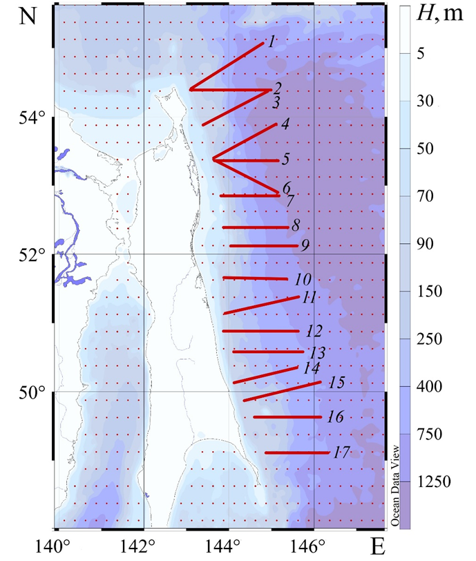
F i g. 1. Geographical location of sections, along which the internal wave dynamics were modeled, in the Sea of Okhotsk
At the first step of the algorithm, the values located on the lines 15 m below the surface and above the bottom were selected from the horizontal velocity field. If we talk about the bottom boundary layer (BBL), its thickness depends on many factors including tidal intensity, bottom slopes and latitudes [18]. A good review of existing empirical models applied for estimating the BBL thickness is given in [19]. It also demonstrates the results of a 15-day observation of the BBL thickness on an area of the continental shelf with a depth of 250 m and sufficiently strong tides (comparable in amplitude to those used in our model). It was revealed that, on average, the BBL was ~ 10 m. We also relied on the BBL estimates obtained by modeling the selected sections using the completely nonlinear nonhydrostatic model for viscous fluids SUNTANS [20]. Although the absence of viscosity in the model we used does not provide a realistic description of the flows arising in the boundary layer, generally, the differences in the wave fields obtained in the inviscid and viscous models will not be significant beyond its limits in subcritical regimes [21]. Guided by symmetry considerations and taking into account that horizon z = −15 m does not fall into the upper pycnocline for all sections, the authors analyzed the velocities at a selected depth of 15 m in the near-surface layer.
Figure 2 gives the example of the x–t diagram of near-surface horizontal velocities on section 16.
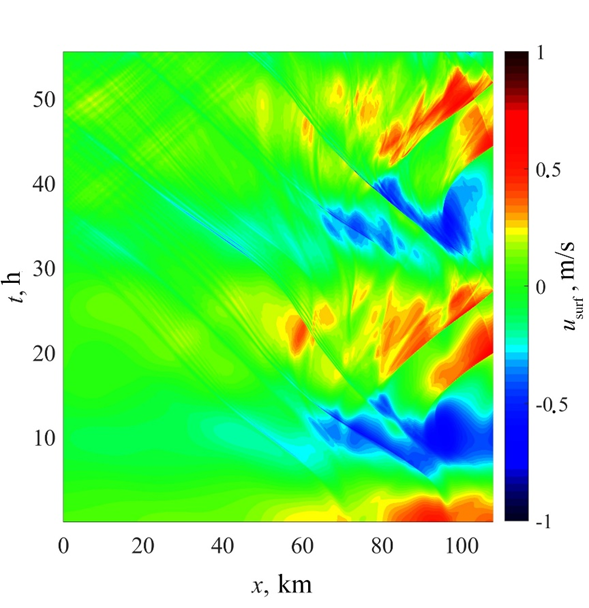
F i g. 2. Spatio-temporal (x–t) diagram for near-surface (fixed at the 15 m depth) velocities on section 16
At the second step of the algorithm, diagrams of probability of level exceeding for the near-surface and near-bottom velocity were constructed allowing for the direction (sign) and according to the absolute value. Then, the velocities at a probability level 0.05, 0.1 and 0.15 were identified and, conversely, the probability with which the velocity 0.25 or 0.3 m/s would be exceeded was determined. The selection of such values is due to the estimates of the threshold velocities at which the displacement of soil particles can be observed. Thus, in [22], a method for determining the nature of bottom sediment movement is given based on the values of the dimensionless Rouse number (Ro), which is defined as the ratio of velocity (Ws) of hydraulic-size suspended particles fall to the dynamic velocity of vertically non-uniform water flow :

where β is ratio of eddy viscosity to eddy diffusion (approximately equal to unity); k is Karman constant (equal to 0.4). Figure 3 represents a nomogram that makes it possible to determine the nature of sediment material movement: when Ro ≥ 7, the sediment movement is initiated by a wave flow and the particles begin to move in the form of rolling; an increase in the flow velocity at 7.5 ≥ Ro ≥ 2.5 leads to the movement of tractional sediments; at 2.5 ≥ Ro ≥ 1.2, saltation of sediment particles occurs; the movement of suspended sediments occurs at 1.2 ≥ Ro ≥ 0.8; intensive movement of bottom sediments, leading to significant deformations of the bottom, occurs at Ro ≤ 0.8 [22].
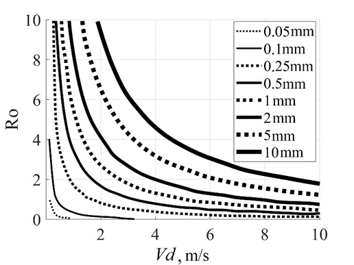
F i g. 3. Nomogram of sediment movement pattern (adapted from [22, p. 379]); Vd is near-bottom wave velocity
Let us use the map of the Sakhalin shelf bottom sediments from the National Atlas of Russia, Volume 2, available at https://nationalatlas.ru/tom2. It is evident that when moving from the coastline to the deep-water part, fine (0.1–0.25 mm in diameter), medium (0.25–0.5 mm) and coarse (0.5–1 mm) sands are replaced by coarse aleurites (0.01–0.05 mm), fine aleuritic silts, clay aleurites and clay silts at the maximum depth. Velocities ~ 0.25 m/s for aleurites are observed at Ro ≤ 0.8, which can lead to significant bottom deformations. Movement of fine and medium bottom sand is also possible, especially under periodic wave action. According to work , erosive velocities for fine sand are 0.2–0.4 m/s, for light sandy soil – 0.3–0.45 m/s; the same threshold velocity values can be found in regulatory documents. Although the baroclinic flow velocity was measured 15 m above the bottom level at the BBL conventional boundary, the same order of velocity values can be observed at the bottom. This is due to the fact that the currents induced by the observed solitons of internal waves reach a maximum velocity at the bottom and surface of the basin, and the model does not consider turbulent flows that can be generated at the bottom.
Figure 4 shows an example of a diagram of near-surface velocities on section 16. The figure also represents a cut of a diagram of exceeding probability of the near-surface velocity level at value 0.25 m/s and a cut according to a probability 0.05. The upper part of the graph corresponds to positive (to coast) velocities, while the lower part corresponds to negative ones. The diagram asymmetry characterizes the wave field complex structure. The absolute values of velocities were also analyzed at each point of the route by the probability and velocity level.
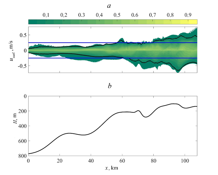
F i g. 4. Diagram of probability of exceeding near-surface (fixed at the 15 m depth) velocity level on section 16 allowing for the sign (direction): blue line is a cut at value 0.25 m/s; black curve is a cut according to a probability 0.05 (a); lower graph shows bottom bathymetry (b)
Maps of threshold values of baroclinic current velocities
We proceed to the analysis of the obtained results. Figure 5 contains the maps of probability levels of the bottom and surface velocities exceeding 0.25 m/s. Local probability maxima are reached in the shelf areas from Cape Elizabeth to the northern boundary of Piltun Bay, from the southern edge of Piltun Bay to Chaivo Bay, opposite Lunskiy Bay and near Cape Bellingshausen. For velocities allowing for the sign and their absolute values, the location of local maxima in the bottom and surface layers coincides. However, for absolute values and velocities directed from the coast, the probabilities in the bottom layer are generally not lower than in the surface layer. For velocities directed to the coast, on the contrary, the probabilities of exceeding the level of 0.25 m/s at the surface are generally not lower than in the bottom layer. In the northern part of the shelf (up to Chaivo Bay), the areas where the probability levels are within 0.8–1 for absolute values and 0.6–0.8 for velocities directed to and from the coast are located. The probabilities of exceeding the level 0.25 m/s reach 0.8 southwards of Chaivo Bay in very small areas for absolute velocities only, and they do not exceed 0.4 for velocities allowing for the sign.
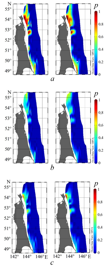
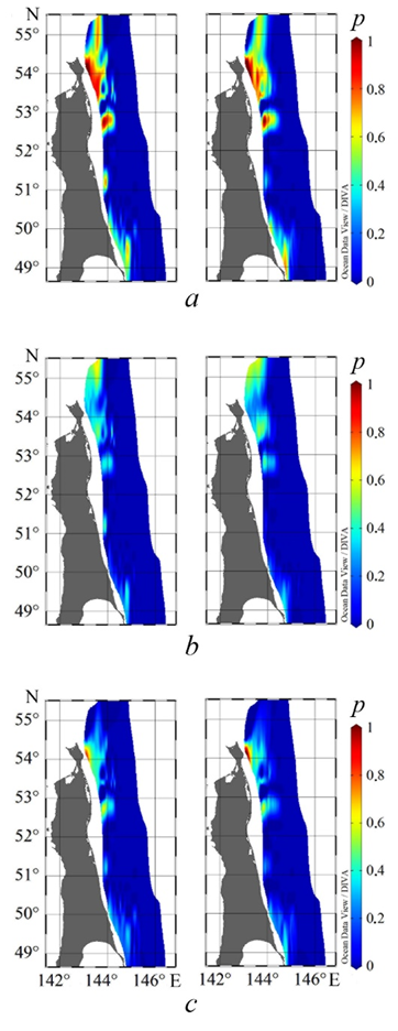
Figure 6 represents the maps of probability levels of exceeding 0.3 m/s for the near-bottom and near-surface velocities. When comparing Figs. 5 and 6, it is clear that the maxima location coincides, although the probabilities are lower; this is especially noticeable for the areas located southwards of Chaivo Bay.
|
|
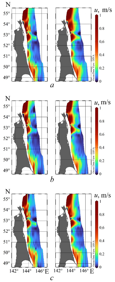
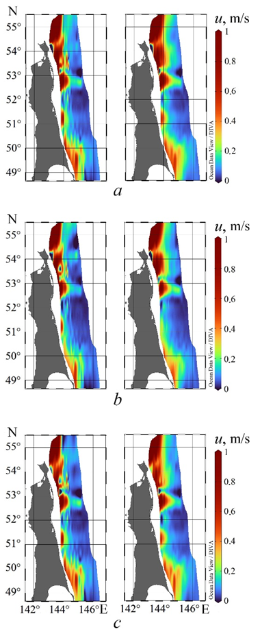
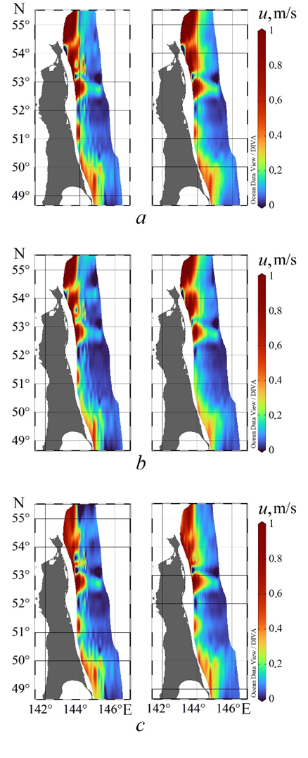
Figures 7–9 show the maps of distribution of the near-surface (15 m from the surface) and near-bottom (15 m above the bottom) velocities by absolute value, directed to and from the coast, that will be exceeded with a probability 0.05; 0.1; 0.15. The main maxima, close to 0.8 m/s, are located in the north – from Cape Elizabeth to Piltun Bay, the second zone of local maxima is in the south – from Cape Bellingshausen to Cape Terpeniya. In the remaining zones, the maximum velocities do not exceed 0.3 m/s. In the upper and lower layers, asymmetry regarding to direction (from or to the coast) is observed: in the northern zones, the velocities directed from the coast decrease significantly in magnitude (Figs. 7, c; 8, c; 9, c) within 1–0.7 m/s with a probability level increase, while in the direction to the coast (Figs. 7, b; 8, b; 9, b), changes are insignificant (velocities of ~ 1 m/s are reached in the bottom and surface layers). In the southern zone, when moving from a probability 0.05 to a level of 0.15, local maxima become less pronounced, especially in the surface layer and in the direction to the coast (velocities of ~ 0.5 m/s are reached only in the bottom layer near Terpeniya Peninsula and Lunskiy Bay).
|
|
F i g. 9. The same as in Fig. 7, at exceeding with a probability 0.15 |
Figures 10–12 represent the scatter diagrams of near-bottom and near-surface velocities by absolute value and allowing for direction depending on the total depth at the section point and the probability level at which these values can be exceeded. It is evident from Fig. 10 that all the diagrams show the maximum scatter of points in the sea areas of up to ~ 500 m depth, and the values of near-bottom and near-surface velocities over 0.5 m/s appear at a total depth of less than 300 m. With a probability level increase, the concentration of points in the upper part of the cloud (where the velocities are over 1 m/s) decreases naturally. At 700–800 m depths, a set of points where the absolute values of near-surface velocities are several times higher than the bottom velocities is clearly expressed. Consideration of velocity direction as well as its measurement depth (bottom or surface layer) increases significantly the scatter of points in the zones of up to 500 m (Fig. 10, d), which indicates the essentially nonlinear nature of currents once again.
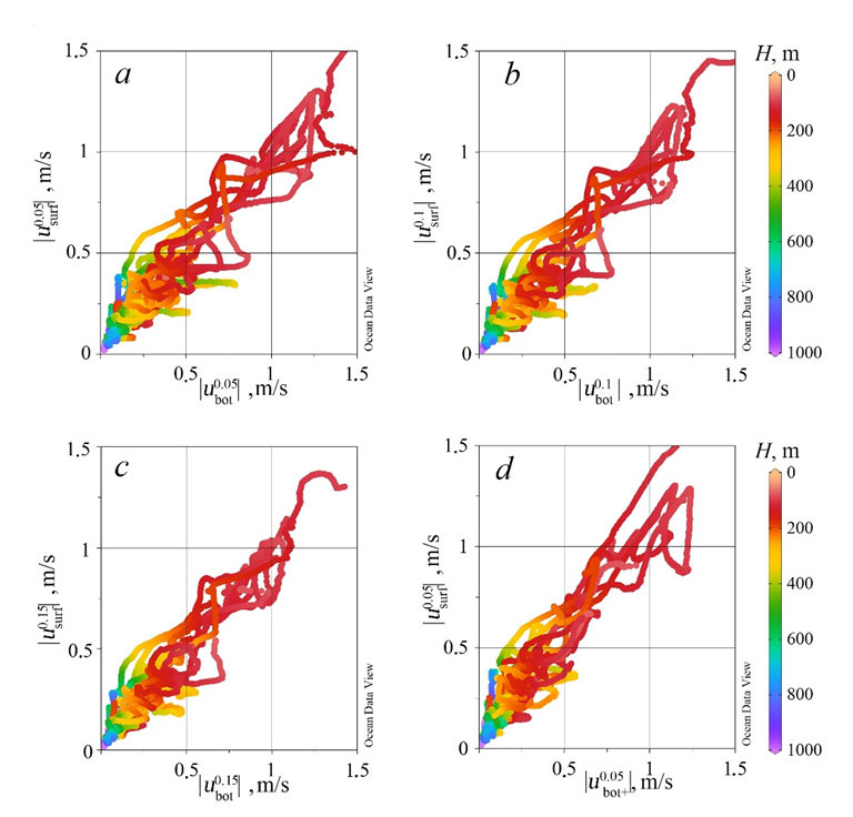
F i g. 10. Scatter plots of absolute values of the near-bottom and near-surface velocities at a probability level 0.05 (a), 0.1 (b) and 0.15 (c), as well as near-bottom velocity to the coast and absolute values of near-surface velocity at a probability level 0.05 (d). Color shows total depth at the point
|
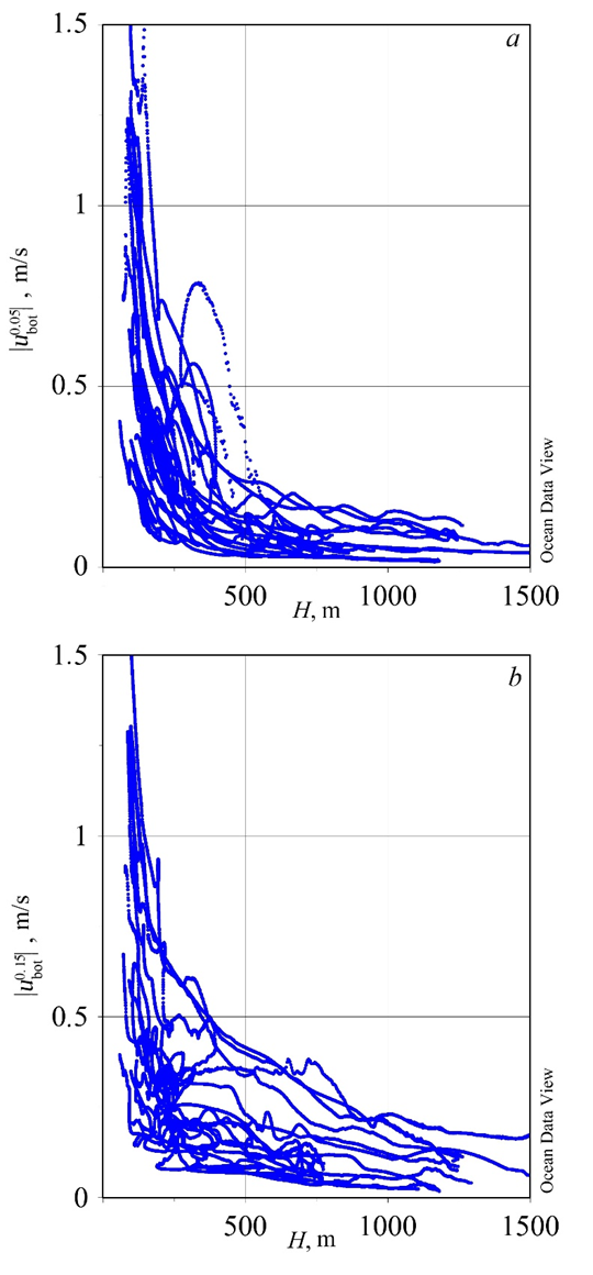
F i g. 11. Dependence of the near-bottom velocity absolute values at a probability level 0.05 (a) and 0.15 (b) upon the total depth at the point |

F i g. 12. Scatter plots of: the near-bottom velocity directed from the coast and the near-surface one – to the coast (a), the near-bottom velocity directed from and to the coast (b), the near-bottom velocity to the coast and the near-surface one – from the coast (c), the near-surface velocity to and from the coast (d), the near-bottom and near-surface velocities to the coast (e), the near-bottom and near-surface velocities from the coast (f) at a probability level 0.15. Color shows total depth at the point. Red line is linear regression
Figure 11 shows the distribution of near-bottom velocities by depth. It is clearly seen that 0.25 m/s velocities and higher are reached only at points with a sea depth of up to 500 m, while at depths from 100 to 500 m, bottom velocities within 0.25–0.5 m/s prevail at probability levels p 0.05 and 0.15.
When studying the correlation dependence of near-bottom/near-surface velocities, the directions (from the coast / to the coast) were taken into account (Fig. 12). When comparing Figs. 12 and 10, we can conclude that a due regard for the direction leads to the fact that the cloud of points in all diagrams becomes wider and the scatter increases. At the same time, the regression coefficient remains close to one in all graphs and is 0.9 (a, c), 0.95 (b), 0.94 (d, e), 0.89 (f) (Fig. 12).
Conclusion
In this work, the spatial structure of baroclinic currents on the northeastern shelf of Sakhalin Island is studied: maps of exceedance probability levels for values 0.25 and 0.3 m/s for the near-bottom (15 m above the bottom level) and near-surface (15 m from the surface) velocities (erosive velocities for fine sand and light sandy soil) by absolute value, directed to and from the coast are constructed and analyzed, as well as maps of the values distribution of the near-surface and near-bottom velocities by their absolute value, in the direction to and from the coast with probability of exceeding of 0.05; 0.1; 0.15. The precalculated horizontal velocity fields were obtained by modeling the dynamics of internal waves using 17 two-dimensional sections under a completely nonlinear model based on the Euler system of equations in the Boussinesq approximation. In all maps, the main local maxima of values are located in the shelf areas from Cape Elizabeth to the northern boundary of Piltun Bay, from the southern edge of Piltun Bay to Chaivo Bay, opposite Lunskiy Bay as well as near Cape Bellingshausen.
It is shown that the horizontal velocity field is essentially nonlinear: asymmetry is visible both in direction (from coast/to coast) and depth (in the bottom and surface layers). To demonstrate this conclusion, scatter plots of various combinations of the near-bottom and near-surface velocities are also constructed in absolute value and allowing for direction. The maximum scatter of points in all the plots is observed at sea depths of up to ~ 500 m, and values of near-bottom and near-surface velocities over 0.5 m/s are traced at depths of less than 300 m. Consideration of velocity direction and measurement depth (near-bottom/near-surface) leads to an increase in the scatter of points and the width of the point cloud cross-section (especially at values higher than 0.3 m/s), which is apparently associated with a complex nonlinear structure of the horizontal velocity field.
1. Maisondieu, C., 2015. WEC Survivability Threshold and Extractable Wave Power. In: A. Clément, ed., 2015. 11th European Wave and Tidal Energy Conference (EWTEC 2015). Nantes, France, 8 p.
2. Arinaga, R.A. and Cheung, K.A., 2012. Atlas of Global Wave Energy from 10 Years of Reanalysis and Hindcast Data. Renewable Energy, 39(1), pp. 49-64. https://doi.org/10.1016/j.renene.2011.06.039
3. Gonçalves, J., Martinho, P. and Guedes Soares, C., 2014. Wave Energy Conditions in the Western French Coast. Renewable Energy, 62, pp. 155-163. https://doi.org/10.1016/j.renene.2013.06.028
4. García-Medina, G., Özkan-Haller, H.T. and Ruggiero, P., 2014. Wave Resource Assessment in Oregon and Southwest Washington, USA. Renewable Energy, 64, pp. 203-214. https://doi.org/10.1016/j.renene.2013.11.014
5. Grigorieva, V.G., Badulin, S.I. and Gulev, S.K., 2022. Global Validation of SWIM/CFOSAT Wind Waves against Voluntary Observing Ship Data. Earth and Space Science, 9(3), e2021EA002008. https://doi.org/10.1029/2021EA002008
6. Shevchenko, G.V. and Besedin, D.E., 2020. Cold-Season Characteristics of Currents off the Northeastern Shelf of Sakhalin Derived from Instrumental Observations. Meteorologiya i Gidrologiya, (6), pp. 87-97 (in Russian).
7. Yarichin, V.G., Vlasov, N.A., Oleinikov, I.S. and Shkileva, A.A., 2012. [Peculiarities of Spatial Variability of Harmonic Constants of Tidal Currents of Diurnal Waves on the Northeastern Shelf of Sakhalin Island (According to the Data of Environmental Monitoring of Oil-and-Gas Areas)]. FERHRI Issues, 154, pp. 145-186 (in Russian).
8. Kolesnikova, A.S., Dubina, V.A., Kruglik, I.A. and Rudenko, O.N., 2022. Satellite Radar Monitoring of Sakhalin Island Shelf. In: FESTFU, 2022. Urgent Problems of the World Ocean Biological Resources Development: Proceedings of the VII International Scientific and Technical Conference. Vladivostok: Far Eastern State Technical Fisheries University, pp. 108-112 (in Russian).
9. Vella, N., Foley, J., Sloat, J., Sandoval, A., D’Attile, L. and Masoumi, M., 2022. A Modular Wave Energy Converter for Observational and Navigational Buoys. Fluids, 7(2), 88. https://doi.org/10.3390/fluids7020088
10. Svergun, E.I., Zimin, A.V., Kulik, K.V. and Frolova, N.S., 2023. Surface Manifestations of Short-Period Internal Waves in the Sea of Okhotsk and the Kuril-Kamchatka Region of the Pacific Ocean. In: T. Chaplina, ed., 2023. Complex Investigation of the World Ocean (CIWO-2023). CIWO 2023. Springer Proceedings in Earth and Environmental Sciences. Cham: Springer, pp. 141-149. https://doi.org/10.1007/978-3-031-47851-2_17
11. Li, J., Zhang, Q. and Chen, T., 2022. ISWFoam: A Numerical Model for Internal Solitary Wave Simulation in Continuously Stratified Fluids. Geoscientific Model Development, 15(1), pp. 105-127. https://doi.org/10.5194/gmd-15-105-2022
12. Rouvinskaya, E.A., Kurkina, O.E. and Kurkin, A.A., 2023. Spatial Distribution of Internal Tidal Waves on the Northeastern Shelf of Sakhalin. Doklady Earth Sciences, 509(1), pp. 148-152. https://doi.org/10.1134/S1028334X22601778
13. Lamb, K.G., 1994. Numerical Experiments of Internal Wave Generation by Strong Tidal Flow across a Finite Amplitude Bank Edge. Journal of Geophysical Research, 99(C1), pp. 843-864. https://doi.org/10.1029/93JC02514
14. Egbert, G.D. and Erofeeva, S.Y., 2002. Efficient Inverse Modeling of Barotropic Ocean Tides. Journal of Atmospheric and Oceanic Technology, 19(2), pp. 183-204. https:/doi.org/10.1175/1520-0426(2002)019<0183:EIMOBO>2.0.CO;2
15. Vlasenko, V., Stashchuk, N. and Hutter, K., 2005. Baroclinic Tides: Theoretical Modeling and Observational Evidence. Cambridge: Cambridge University Press, 351 p. https://doi.org/10.1017/CBO9780511535932
16. Rouvinskaya, E.A., Kurkina, O.E. and Kurkin, A.A., 2021. [Particle Transport and Dynamic Effects during of a Baroclinic Tidal Wave Transformation in the Conditions of the Shelf of the Far Eastern Seas]. Ecological Systems and Devices, (11), pp. 109-118. https:/doi.org/10.25791/esip.11.2021.1270 (in Russian).
17. Kuznetsov, P.D., Rouvinskaya, E.A., Kurkina, O.E. and Kurkin, A.A., 2021. Transformation of Baroclinic Tidal Waves in the Conditions of the Shelf of the Far Eastern Seas. In: IOP, 2021. IOP Conference Series: Earth and Environmental Science. Vol. 946, 012024. https:/doi.org/10.1088/1755-1315/946/1/012024
18. Holloway, P.E. and Barnes, B., 1998. A Numerical Investigation into the Bottom Boundary Layer Flow and Vertical Structure of Internal Waves on a Continental Slope. Continental Shelf Research, 18(1), pp. 31-65. https://doi.org/10.1016/s0278-4343(97)00067-8
19. Zulberti, A.P., Jones, N.L., Rayson, M.D. and Ivey, G.N., 2022, Mean and Turbulent Characteristics of a Bottom Mixing-Layer Forced by a Strong Surface Tide and Large Amplitude Internal Waves. Journal of Geophysical Research: Oceans, 127(1), e2020JC017055. https://doi.org/10.1029/2020JC017055
20. Kuznetsov, P.D., Rouvinskaya, E.A., Kurkina, O.E. and Kurkin, A.A., 2023. Approximate Estimates of the Force Impact of Baroclinic Flows on Cylindrical Supports in the Conditions of the Sakhalin Shelf. Ecological Systems and Devices, (10), pp. 56-66. https://doi.org/10.25791/esip.10.2023.1406 (in Russian).
21. Soontiens, N., Stastna, M. and Waite, M., 2015. Topographically Generated Internal Waves and Boundary Layer Instabilities. Physics of Fluids, 27(8), 086602. https://doi.org/10.1063/1.4929344
22. Kuznetsova, M.N. and Plink, N.L., 2018. Methodological Calculations for the Preliminary Evaluation of Sediment Transport Characteristics. In: IO RAS, 2018. Proceedings of the II Russian National Conference “Hydrometeorology and Ecology: Scientific and Educational Achievements and Perspectives”. Saint Petersburg: Himizdat, pp. 377-380 (in Russian).