Introduction

Atmospheric pressure variations significantly contribute to the oscillations and waves that occur in the hydrosphere. Passage of tropical cyclones and typhoons over small bays leads to an increase in the amplitudes of eigen oscillations of seas and their separate parts [1–3].

Amplitudes of seiches in bays and seas can increase when acoustic-gravity waves pass over a water area. This phenomenon occurred during the explosion of the volcano in January 2022, when the eruption on Hunga Tonga-Hunga Haʻapai Island in the Tonga archipelago escalated to the active explosive phase. An acoustic-gravity Lamb wave was formed, which circled the Earth several times [4]. Analysis of data from wave recorders installed in the Sea of Japan revealed an increase in the amplitudes of seiches both in the sea itself and in the bays where the recorders were installed [5]. The reason for the growth of seish was the disturbance that occurred in the atmosphere. An abrupt change in atmospheric pressure in some cases leads to the formation of a wave with characteristics similar to a tsunami. This is a meteorological tsunami, or meteotsunami, caused not by underwater earthquakes and landslides, but by atmospheric processes passing over the ocean [6]. Sometimes, a meteorological tsunami occurs during the passage of a thunderstorm front, which can be caused by atmospheric gravity waves or an abrupt change in wind direction over the water surface.

Resonance effects play an important role in the generation of meteotsunamis when the period of eigen oscillations of the water area and their propagation velocity are close to the period and propagation velocity of atmospheric disturbances. However, not every atmospheric front or atmospheric disturbance leads to the generation of a meteorological tsunami. The most important is the atmospheric pressure gradient, which directly affects the ocean [7].

As observations show, the consequences of meteorological tsunamis can be serious and, in some regions, even catastrophic. For example, in June 2014 in Croatia, the water level in the harbor began to rise, resulting in flooding of the roads, displacement of cars and landing of boats onshore. Over time, the water receded from the streets. However, there were no strong underwater earthquakes at the time. Similar destructive meteorological tsunamis have been observed on the shores of the Yellow and Black Seas. The majority of cases of destructive waves, not associated with seismic events, have been recorded along the coasts of Japan, Europe and North America.

There is no periodicity in the occurrence of meteorological tsunamis, in some areas they occur only in spring and summer months, while in others, they occur once every 3–5 years [8–12]. During the registration of a meteotsunami, increases in the amplitude of sea excitement are also observed in the range of periods from 2 minutes to 3 hours [13]. Water levels rise very slowly during a meteorological tsunami, within tens of minutes or even hours. The water can rise by a few decimeters or even several meters, flooding areas close to the basin and altering the coastline [14]. The consequences of such natural disasters can be enormous, although not comparable to ordinary tsunamis. The development of measuring equipment over the past 30 years has almost doubled the proportion of meteotsunamis recorded. In order to assess and prevent the consequences of meteorological tsunamis, the databases are used to develop numerical models to evaluate the impact of an abrupt change in atmospheric pressure on the water surface [15–17].

According to the data of experimental observations of near-bottom hydrostatic pressure conducted by Russian scientists from the Institute of Marine Geology and Geophysics of the Far Eastern Branch of the Russian Academy of Sciences in the shelf area of the southern part of Sakhalin Island and the Kuril Islands, sea level fluctuations corresponding to tsunami waves were identified. Analysis of the seismic situation in this area showed that there were no strong underwater earthquakes on these days, and these fluctuations were attributed to meteorological tsunamis [18].

Meteotsunami phenomena are actively studied by scientists around the world. In most cases, meteorological stations and tide sensors are used to register meteotsunamis. In some cases, wave gauges and mareographs are used. Based on data from meteorological stations and tide sensors in the Yellow Sea, scientists identified 42 events from 2010 to 2019 that can be attributed to a meteotsunami [16, 19]. This phenomenon is often found off the coast of Japan, which is recorded by deep-sea sensors of the DART (Deep-ocean Assessment and Reporting of Tsunamis) type. Based on measurements from meteorological stations, wave detectors and deep-sea sensors, the trajectory of the meteotsunami wave and possible consequences are calculated [20, 21]. This approach is essential for reducing possible consequences when a meteotsunami wave comes ashore.

In the south of the Primorsky Territory, in Posyet Bay, according to the data of laser-interference devices and a broadband seismograph, a natural phenomenon was recorded. This phenomenon exhibited characteristics consistent with meteotsunami. Specifically, the data from the laser nanobarograph indicated an atmospheric disturbance of several hPa, which led to the emergence of anomalous solitary hydrosphere waves with amplitudes several times higher than the amplitudes of irregular semi-diurnal fluctuations typically observed in this region [22]. These waves were recorded by the laser meter of hydrosphere pressure variations, which was installed on the shelf of the Sea of Japan. During the solitary wave recordings, an increase in the amplitude of oscillations with periods ranging from 2 to 2.5 minutes was observed in the recordings of laser strainmeters. A few hours after the registration of waves in the hydrosphere, fluctuations with a period of approximately one and a half hours were detected in the recordings of the laser strainmeter and the laser nanobarograph. The present article describes this phenomenon and offers a probable assessment of its manifestation in the neighboring geospheres (atmosphere, hydrosphere, lithosphere).

Materials and methods

Since the year 2000, a seismoacoustic hydrophysical complex has been operating continuously on the base of the Cape Schultz Marine Experimental Station of the V.I. Il’ichev Pacific Oceanological Institute of FEB of RAS. The complex includes laser strainmeters, a laser nanobarograph, laser meters of hydrosphere pressure variations, a broadband seismograph, a weather station, a laboratory room, and auxiliary equipment.

All laser meters are based on Michelson interferometers using a frequency-stabilized helium-neon laser with a long-term stability frequency of 10⁻⁹ as a light source. The laser strainmeters are based on Michelson unequal-arm interferometers with measuring arm lengths of 52.5 and 17.5 m and North-South and West-East orientations, respectively. Both strainmeters are capable of detecting microdeformations of the Earth’s crust in the frequency range from 0 (conditionally) to 1000 Hz, with an accuracy of 0.3 nm and an almost unlimited dynamic range [23]. The laser nanobarograph is based on Michelson equal-arm interferometer, where the aneroid box is the sensitive element. The device is capable of detecting atmospheric pressure variations in the frequency range from 0 (conditionally) to 1000 Hz with an accuracy of 1 μPa and in an almost unlimited dynamic range [24]. The laser meter of hydrosphere pressure variations is made on the basis of a nonequal-arm Michelson interferometer using a thin membrane fixed at the edges as a sensitive element. The meter is capable of detecting hydrosphere pressure variations in the frequency range from 0 (conditionally) to 1000 Hz with an accuracy of 1 μPa and in an almost unlimited dynamic range [25]. The complex also includes a Guralp CMG-3ESPB broadband seismograph with an operating frequency range f 0.003–50 Hz per sensor. Data from all devices are transmitted via cable lines to the laboratory room, where a database of experimental data is created after preliminary processing.

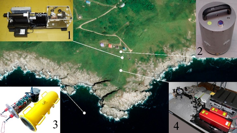
F i g. 1. Device arrangement scheme: 1 – laser nanobarograph; 2 – broadband seismograph; 3 – laser meter of hydrosphere pressure variations; 4 – laser strainmeter

Figure 1 shows the arrangement of the devices included in the complex. Laser strainmeters are installed under the Earth’s surface at a distance of 80 m from each other. Optical parts of the interferometers are installed in thermally insulated rooms to eliminate the influence of temperature variations on the instrument measurements. The broadband seismograph is installed below the surface in a thermally insulated chamber between two laser strainmeters. The laser nanobarograph is installed in a thermally insulated room 50 m from the laser strainmeter with North-South orientation and about 30 m from the laser strainmeter with West-East orientation. The laser meter of hydrosphere pressure variations is installed on the shelf of the Sea of Japan at a distance of 200 m from the coast and 300 m from the 52.5 m laser strainmeter at a depth of 33 m.

In the course of solving the aforementioned problems, we performed processing and analysis of synchronous experimental data obtained during the registration of atmospheric pressure variations by laser nanobarographs, hydrostatic pressure variations by laser hydrosphere pressure meters and microdeformations of the upper layer of the Earth’s crust by laser strainmeters. To assess the meteotsunami manifestation in neighboring geospheres, we shall consider synchronous data for May 2015. The data records of all laser interference meters were obtained with a duration of 1 hour and a sampling rate of 1000 Hz. For convenience, the data were filtered with a low-frequency Hamming filter up to 1 Hz and diluted 1000-fold. As a result, we obtain a set of data from laser strainmeters, the laser nanobarograph and the laser meter of hydrosphere pressure variations with a sampling rate of 1 Hz. The measurement of the main parameters of oscillations and waves in all geospheres is carried out simultaneously, which, with their subsequent processing, makes it possible to determine more accurately the primary source in the “atmosphere-hydrosphere-lithosphere” system.

Results and discussion

Registration and analysis of atmospheric-hydrosphere oscillations. Processing the data of atmospheric pressure variations obtained by the laser nanobarograph and hydrostatic pressure obtained by the laser hydrosphere pressure change meter, several events of abnormal hydrosphere behavior were detected on May 25–26, 2015. The laser nanobarograph recorded an abrupt change in atmospheric pressure (Fig. 2) with a magnitude of 13.5 hPa. The abrupt change in atmospheric pressure was recorded at 15:20 on May 25, 2015. The abrupt change in atmospheric pressure was also accompanied by an increase in oscillations with periods of 2 to 2.5 min.

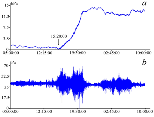
F i g. 2. Fragment of the laser nanobaroghraph recording for May 25–26, 2015, UTC (a) (adapted from [22]) and filtered fragment of the laser nanobaroghraph recording (b)

To identify these oscillations, we filter the laser nanobarograph recording with a bandpass filter. The recording clearly shows an increase in the amplitudes of these oscillations at the time of registration of the atmospheric pressure increase (Fig. 2, b). The amplitudes of oscillations with periods of 2 to 2.5 min increased almost tenfold. After the atmospheric pressure stabilized, these oscillations also decreased. Such an increase in atmospheric pressure could be attributed to the arrival of a typhoon or cyclone at the site where the instruments were installed. However, according to the Meteorological Service of the Russian Academy of Sciences, no cyclones or, especially, typhoons were recorded in the region at that time. The weather over the region was clear with moderate northeasterly winds.

Let us look at the records of the laser meter of hydrosphere pressure variations at the time of registration of the atmospheric pressure increase and after this increase. Figure 3 shows a record of the laser interference meter installed on the bottom in the shelf zone of the Sea of Japan at a depth of 33 m on May 25–26, 2015. The initial disturbance was recorded almost an hour and a half after the start of registration of the atmospheric pressure jump. The registration of the initial disturbance began at 16:44 on May 25, 2015, and almost 12 hours later, at 04:20 on May 26, 2015, the second disturbance was recorded.

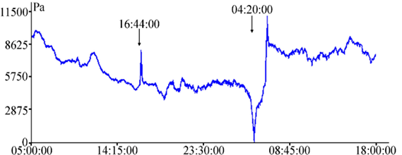
F i g. 3. Fragment of the recording of the laser meter of hydrosphere pressure variations for May 25–26, 2015, UTC (adapted from [22])

The two disturbances were inherently different. If the first was a solitary wave of almost soliton-like shape (Fig. 4, a), the second was a wave accompanied by an outflow of water masses (Fig. 4, b). The first wave caused only an inflow of water masses (increase of hydrostatic pressure) and its characteristics were very similar to a tsunami wave. The height of the recorded wave was four times higher than the amplitude of the irregular semi-diurnal tide in this region. The amplitude of the 9irregular semi-diurnal tide according to the sea level station monitoring facility was 0.1 m . The wave propagation time through the point, where the laser meter of hydrosphere pressure variations was installed was about 14.5 min. During the arrival of the second wave, the first outflow of water masses was recorded (decrease of hydrostatic pressure). The depth of the sea at the location of the device decreased by a value approximately equal to five amplitudes of the irregular semi-diurnal tide. The outflow of water masses lasted 25.5 min, and then the sea level returned to its previous position within 16 min. The third wave was recorded by the laser meter of hydrosphere pressure variations in about an hour. As with the arrival of the first wave, an influx of water masses was observed. However, their shapes were different, and the wave height was almost double that of the height of the first wave. The graph shows that the sea level began to rise sharply, and in 5 min, a decrease of one third of this value began. Nevertheless, with the arrival of another wave, the hydrostatic pressure begins to rise again. The total time of wave propagation through the installation point of the laser meter of hydrosphere pressure variations was 23 min.

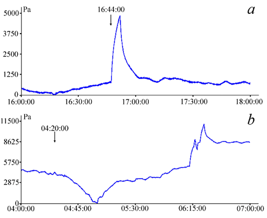
F i g. 4. Enlarged fragments of the recordings of the laser meter of hydrosphere pressure variations for May 25, 2015, UTC (a) and May 26, 2015, UTC (b) (adapted from [22])

Hen recording these solitary waves, the initial sea level did not change until after the arrival of the third wave. If the sea level recovered immediately after the first wave, it returned to its initial position 40 min after the second wave. After the third wave, the sea level rose, and it took several days for the sea level to return to its initial state. Considering that the time of the first disturbance passage was 14.5 min, the total period of the wave should be approximately 29 min. This is close to the period of seiches of the Sea of Japan, recorded in the region, which is 30.5 min [26]. However, upon analyzing the second and the third disturbances, it is evident that the total period of the waves is 51 and 46 min respectively, which is much longer than the seiche period observed in the region. In terms of their shape, the second and the third waves differ from the first, as they are not as well defined. In the third case, there is an apparent overlap of the waves. The registration of solitary waves, instead of the increase in the amplitudes of the Sea of Japan seiches, testifies to the fact that the increase in atmospheric pressure did not take place over the entire area of the sea, but formed in its certain part and then moved towards the site of installation of the laser interference devices. Taking into account that the registration of the atmospheric disturbance began 1 hour 24 min earlier than the disturbance in the hydrosphere, we can say that it caused solitary waves in the hydrosphere.

Similar behavior of water masses was recorded in 1978 in Vela Luka, Croatia. Early in the morning, the water began to come into the streets of the city, flooding everything in its path, and after 10 min it began to move back. After some time, the phenomenon repeated itself. The flood in Vela Luka is considered one of the most striking examples of the phenomenon, which has been called a “meteorological tsunami” (or simply “meteotsunami”) . In this context, the solitary waves recorded by the laser meter of hydrosphere pressure variations, along with the increase in atmospheric pressure, recorded by the laser nanobarograph, can be associated with a meteorological tsunami.

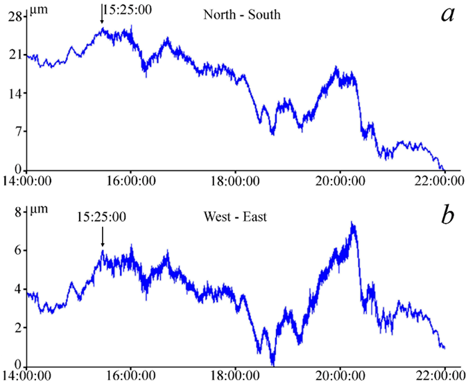
F i g. 5. Fragments of the laser strainmeter recordings, North-South orientation (a), West-East orientation (b) for May 25, 2015, UTC (adapted from [22])

Registration and analysis of lithospheric oscillations. During the arrival of atmospheric disturbance recorded by the laser nanobarograph, oscillations of the earth crust with periods from 2 to 2.5 min are observed on the recordings of laser strainmeters and the broadband seismograph. Figure 5 shows fragments of recordings of the laser strainmeter with measuring arm length of 52.5 m and North-South (a) orientation and the laser strainmeter with measuring arm length of 17.5 m and West-East orientation (b). Both graphs show that at approximately 3:20 p.m. on May 25, 2015, micro deformations of the earth crust begin to appear with periods from 2 to 2.5 min, and their amplitude increases. And at the moment of termination of short-period oscillations in the atmosphere, the amplitude of these oscillations in the upper layer of the earth's crust drops to the background level.

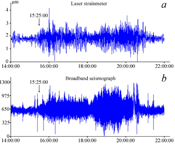
F i g. 6. Filtered fragment of the recording of the laser strainmeter of North-South orientation (a) and fragment of the broadband seismograph recording (b) for May 25, 2015, UTC (adapted from [22])

When analyzing the broadband seismograph data, an increase in the amplitude of crustal oscillations with periods of 2 to 2.5 min is also observed. Thus, Fig. 6 shows a fragment of the broadband seismograph recording of the North-South arm (bottom), where an increase in the amplitude of these oscillations is observed. To compare the laser strainmeter and broadband seismograph records, we filter out the laser strainmeter recording in the frequency range of the seismograph. We use a Hamming bandpass filter with boundaries from 0.003 to 50 Hz. After filtering the fragment of the laser strainmeter recording with North-South orientation, the manifestation of microdeformations within the Earth’s crust with periods from 2 to 2.5 min becomes more pronounced (Fig. 6, a). After filtering, the laser strainmeter and broadband seismograph recordings became similar. A similar manifestation of the crustal oscillations is observed on the horizontal laser strainmeter with West-East orientation and a measuring arm length of 17.5 m, as well as a component of the West-East arm of the broadband seismograph (Fig. 7).

Let us analyze the records of the laser nanobarograph, laser strainmeters, and the broadband seismograph during registration of infragravity oscillations with periods from 2 to 2.5 min. In the laser nanobarograph records, the amplitude of the excited oscillations is 9.3 times greater than the amplitudes of the same oscillations before the atmospheric disturbance. In the records of the laser strainmeters at the moment of the atmospheric disturbance, the amplitude of the oscillations is 9.2 times greater than the amplitudes of the oscillations before the disturbance. Similar values of the ratio of the amplitudes of the oscillations before the atmospheric disturbance and at the time of its registration are observed on the records of the broadband seismograph, the ratio of the amplitudes is 9.4. The atmospheric disturbance, registered by the laser nanobarograph, caused an almost 10-fold increase in the amplitudes of infragravity oscillations in the atmosphere and lithosphere. The similarity of the amplitude ratio of these oscillations does not allow to unambiguously identify their primary source, whether in the atmosphere or in the lithosphere.

F i g. 7. Filtered fragment of the recording of the laser strainmeter with West-East orientation (a) and fragment of the broadband seismograph recording (b) for May 25, 2015, UTC

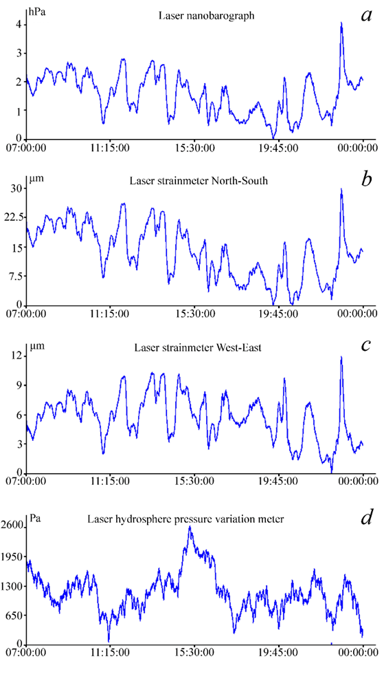
F i g. 8. Fragments of the recordings of laser nanobarograph (a), laser strainmeter with North-South orientation (b), laser strainmeter with West-East orientation (c) and laser meter of hydrosphere pressure variations for May 26–27, 2015, UTC (adapted from [22])

Registration of one and a half hour fluctuations in geospheres. When analyzing the data from the laser-interference devices, oscillations with a period of about one and a half hours were recorded. Consequently, on the recordings of laser strainmeters for May 26 and 27, 2015, oscillations with a period of 1 h 37 min were detected. Figure 8 shows fragments of recordings obtained with laser strainmeters, with measuring arm lengths of 52.5 m (b) and 17.5 m (c). Powerful hour-and-a-half oscillations are observed in both graphs. When processing recordings of the laser nanobarograph installed in close proximity to laser strainmeters, oscillations with similar periods were also identified (Fig. 8, a). A subsequent analysis of hydrostatic pressure data obtained using the laser meter of hydrosphere pressure variations showed the presence of oscillations with similar periods. However, these oscillations are less pronounced in the neighboring geospheres (Fig. 8, d). The correlation coefficient of variations in the pressure of the hydrosphere and the atmosphere is 0.14, and between variations in the pressure of the hydrosphere and microdeformations of the upper layer of the Earth’s crust is 0.22. A more pronounced correlation, with a coefficient of 0.89, is observed between atmospheric pressure variations and micro-deformations of the Earth’s crust. The presence of oscillations with a period of 1 h 37 min in the atmosphere, lithosphere, and hydrosphere indicates their common origin associated with one of the geospheres. The use of complex research methods, integrating laser-interference meters across three distinct geospheres, allows us to determine the primary source of these oscillations. The analysis of the data from the laser nanobarograph, laser strainmeters and the laser meter of hydrosphere pressure variations revealed that the maximum ratio of the amplitude of the hour-and-a-half oscillations to background oscillations in the atmosphere is greater than in other geospheres. The most important factor in determining the primary source is the abrupt change in atmospheric pressure that preceded the arrival of solitary long waves in the hydrosphere. Consequently, it can be concluded that the atmosphere is the primary source of all observed oscillations and waves.

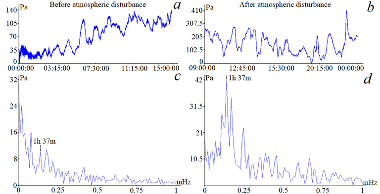
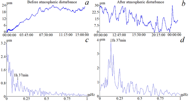
F i g. 9. Fragments and spectra of the laser nanobarograph recordings for May 25 and 26, 2015, UTC

In order to estimate the amplitudes of these oscillations, the spectra of the recordings of the laser nanobarograph and the horizontal laser strainmeters with North-South and West-East orientations must be considered. Figures 9, 10 and 11 illustrate fragments of the recordings and spectra. The left side exhibits the curves prior to the oscillations, while the right side displays the curves at the moment of their arrival.

F i g. 10. Fragments and spectra of the recordings of the laser strainmeter with North-South orientation for May 25 and 26, 2015, UTC

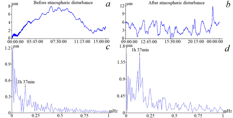
F i g. 11. Fragments and spectra of the recordings of the laser strainmeter with West-East orientation for May 25 and 26, 2015, UTC

Spectra were calculated using sections of recordings of laser interference devices with a duration of 15 h. The recording was made at a frequency of 10 Hz. This results in a duration of 540,000 points for each section. The spectrum of the recording area prior to the atmospheric disturbance exhibited a classical form, accompanied by a few prominent peaks. This spectrum can be attributed to background fluctuations that are constantly present on the instrument recordings. Three peaks with periods of 1 h 23 min, 1 h 37 min and 1 h 49 min are clearly distinguished in the right spectra. The amplitude of the oscillations with a period of 1 h 37 min is the largest, as evidenced by both the instrument recordings and the spectra. A visual analysis of the spectra shows that the amplitudes of these oscillations have increased by more than threefold compared to the background oscillations, thereby becoming more pronounced. Furthermore, the amplitude of these oscillations increased with a period of about 1 h, manifesting as a peak positioned to the right of the group of peaks described above.

Let us compare the oscillations amplitudes with a period of 1 h 37 min before and after the arrival of the atmospheric disturbance. The following Table presents the values of the amplitudes of these oscillations based on the data collected by laser interference devices. The analysis of the data reveals that the maximum ratio of the amplitudes of these oscillations in the spectra of the laser nanobarograph records is nearly 15% higher than in the spectra of the laser strainmeter records. In the context of baro-deformation interaction, atmospheric pressure variations predominantly influence the microdeformations of the Earth’s crust [25]. Consequently, the primary source of the oscillations with a period of 1 h 37 min, as recorded by laser interference devices, is attributed to atmospheric fluctuations. The oscillations with similar periods were identified in the atmosphere several hours after the meteotsunami occurrence in other regions [8].

Value of oscillation amplitudes with a period of 1 h 37 min on laser interference devices

Conclusion

An abrupt increase in atmospheric pressure resulted in the generation of solitary long waves in the hydrosphere, as recorded at 15:20 on May 25. Several waves were recorded by the laser meter of hydrosphere pressure variations. The first wave exhibited a shape resembling a soliton. The first wave’s registration occurred at 16:44 on May 25, while the second wave was recorded at 04:20 on May 26. The time difference between the arrivals of these waves was about 13 hours, and the height of these waves was several times greater than the amplitude of the daily tide in this region. The height of the first wave, which was smaller than the subsequent ones, and its smoother shape indicate that it formed closer to the location of the device. An abrupt change in atmospheric pressure caused an increase in the amplitudes of the oscillations of the infragravity waves. A study of the data from the laser strainmeters and the broadband seismograph revealed an increase in the amplitude of microdeformations of the Earth’s crust with periods ranging from 2 to 2.5 min coinciding with the abrupt change in atmospheric pressure. The registration of changes in the amplitude of these upper layer crust oscillations occurred at 15:25 on May 25. The duration of this change was approximately 6.5 h. Several hours after the passage of the last wave, the records of all laser interference devices revealed the presence of oscillations with a period of approximately one and a half hours. Concurrently, at about 07:00 on May 26, the registration of vibrations and waves with a period of 1 h 37 min commenced simultaneously in all geospheres. However, the largest ratio of the amplitudes of these oscillations before and after the atmospheric disturbance was observed in the atmosphere.

A comprehensive analysis of the data from the laser nanobarograph, laser meter of hydrosphere pressure variations, laser strainmeters, and the broadband seismograph showed that all these disturbances were associated with the passage of meteorological tsunamis in the southern region of the Russian Far East. An abrupt increase in atmospheric pressure, formation of solitary waves in the hydrosphere, an increase in the amplitude of waves with periods from 2 to 120 min are the cause and effect of the passage of meteotsunamis at the location of laser interference devices.

1. Deng, G., Xing, J., Sheng, J. and Chen, S., 2022. A Process Study of Seiches over Coastal Waters of Shenzhen China after the Passage of Typhoons. Journal of Marine Science and Engineering, 10(3), 327. https://doi.org/10.3390/jmse10030327

2. Fan, G. and Xu, Y., 2014. Seiche Phenomenon and the Cause Analysis in the Sea Area of Laohutan of Dalian. Transactions of Oceanology and Limnology, 4, pp.139-143.

3. Dolgikh, S., Dolgikh, G., Zaytsev, A. and Pelinovsky, E., 2023. The Long Wave Height Distribution at the Sea of Japan Caused by Hinnamnor Typhoon Passage: Observations and Modeling. Physical Oceanography, 30(6), pp. 747-759.

4. Xu, J., Li, D., Bai, Z., Tao, M. and Bian, J., 2022. Large Amounts of Water Vapor Were Injected into the Stratosphere by the Hunga Tonga–Hunga Ha’apai Volcano Eruption. Atmosphere, 13(6), 912. https://doi.org/10.3390/atmos13060912

5. Dolgikh, G.I., Dolgikh, S.G. and Ovcharenko, V.V., 2022. Initiation of Infrasonic Geosphere Waves Caused by Explosive Eruption of Hunga Tonga-Hunga Haʻapai Volcano. Journal of Marine Science and Engineering, 10(8), 1061. https:// doi.org/10.3390/jmse10081061

6. Rabinovich, A.B. and Monserrat, S., 1998. Generation of Meteorological Tsunamis (Large Amplitude Seiches) near the Balearic and Kuril Islands. Natural Hazards, 18(1), pp. 27-55. https://doi.org/10.1023/A:1008096627047

7. Ranguelov, B.K., 2011. Natural Hazards-Nonlinearities and Risk Assessment. Sofia, Bulgaria: Prof. Marin Drinov Academic Publishing House, 326 p.

8. Monserrat, S., Vilibić, I. and Rabinovich, A.B., 2006. Meteotsunamis: Atmospherically Induced Destructive Ocean Waves in the Tsunami Frequency Band. Natural Hazards and Earth System Sciences, 6(6), pp. 1035-1051. https://doi.org/10.5194/nhess-6-1035-2006

9. Rabinovich, A.B., 2009. Seiches and Harbor Oscillations. In: Young C. Kim, ed., 2009. Handbook of Coastal and Ocean Engineering. Los Angeles, USA: California State University, pp. 193-236. https://doi.org./10.1142/9789812819307_0009

10. Pattiaratchi, C.B. and Wijeratne, E.M.S., 2015. Are Meteotsunamis an Underrated Hazard? Philosophical Transactions of the Royal Society A, 373(2053), 20140377. https://doi.org/10.1098/rsta.2014.0377

11. Picco, P., Schiano, M.E., Incardone, S., Repetti, L., Demarte, M., Pensieri, S. and Bozzano, R., 2019. Detection and Characterization of Meteotsunamis in the Gulf of Genoa. Journal of Marine Science and Engineering, 7(8), 275. https://doi.org/10.3390/jmse7080275

12. Maramai, A., Brizuela, B. and Graziani, L., 2022. A Database for Tsunamis and Meteotsunamis in the Adriatic Sea. Applied Sciences, 12(11), 5577. https://doi.org/10.3390/app12115577

13. Anarde, K., Figlus, J., Sous, D. and Tissier, M., 2020. Transformation of Infragravity Waves during Hurricane Overwash. Journal of Marine Science and Engineering, 8(8), 545. https://doi.org/10.3390/jmse8080545

14. Kilibarda, Z. and Kilibarda, V., 2022. Foredune and Beach Dynamics on the Southern Shores of Lake Michigan during Recent High Water Levels. Geosciences, 12(4), 151. https://doi.org/10.3390/geosciences12040151

15. Heo, K.-Y., Yoon, J.-S., Bae, J.-S. and Ha, T., 2019. Numerical Modeling of Meteotsunami–Tide Interaction in the Eastern Yellow Sea. Atmosphere, 10(7), 369. https://doi.org/10.3390/atmos10070369

16. Kwon, K., Choi, B.-J., Myoung, S.-G. and Sim, H.-S., 2021. Propagation of a Meteotsunami from the Yellow Sea to the Korea Strait in April 2019. Atmosphere, 12(8), 1083. https://doi.org/10.3390/atmos12081083

17. Kakinuma, T., 2022. Tsunamis Generated and Amplified by Atmospheric Pressure Waves Due to an Eruption over Seabed Topography. Geosciences, 12(6), 232. https://doi.org/10.3390/geosciences12060232

18. Kovalev, P.D., Shevchenko, G.V., Kovalev, D.P. and Shishkin, A.A., 2017. Meteotsunamis on Sakhalin and the South Kuriles. Vestnik of Far Eastern Branch of Russian Academy of Sciences, 1, pp. 79-87 (in Russian).

19. Kim, M.-S., Woo, S.-B., Eom, H. and You S.H., 2021. Occurrence of Pressure-Forced Meteotsunami Events in the Eastern Yellow Sea during 2010-2019. Natural Hazards and Earth System Science, 21(11), pp. 3323-3337. https://doi.org/10.5194/nhess-21-3323-2021

20. Asano, T., Yamashiro, T. and Nishimura, N., 2012. Field Observations of Meteotsunami Locally Called “Abiki” in Urauchi Bay, Kami-Koshiki Island, Japan. Natural Hazards, 64(2), pp. 1685-1706. https://doi.org/10.1007/s11069-012-03330-2

21. Kubota, T., Saito, T., Chikasada, N.Y. and Sandanbata, O., 2021. Meteotsunami Observed by the Deep-Ocean Seafloor Pressure Gauge Network off Northeastern Japan. Geophysical Research Letters, 48(21), e2021GL094255. https://doi.org/10.1029/2021GL094255

22. Dolgikh, S.G. and Dolgikh, G.I., 2019. Meteotsunami Manifestations in Geospheres. Izvestiya, Physics of the Solid Earth, 55(5), pp. 801-805. https://doi.org/10.1134/S1069351319050045

23. Dolgikh, G.I., Valentin, D.I., Dolgikh, S.G., Kovalev, S.N., Koren, I.A., Ovcharenko, V.V. and Fishchenko, V.K., 2002. Application of Horizontally and Vertically Oriented Strainmeters in Geophysical Studies of Transitional Zones. Izvestiya, Physics of the Solid Earth, 38(8), pp. 686-689.

24. Dolgikh G.I., Dolgikh, S.G., Kovalev, S.N., Koren, I.A., Novikova, O.V., Ovcharenko, V.V., Okuntseva, O.P., Shvets, V.A., Chupin, V.A. [et al.], 2004. A Laser Nanobarograph and Its Application to the Study of Pressure-Strain Coupling. Izvestiya, Physics of the Solid Earth, 40(8), pp. 683-691.

25. Dolgikh, G.I., Dolgikh, S.G., Kovalev, S.N., Chupin, V.A., Shvets, V.A. and Yakovenko, S.V., 2009. Super-Low-Frequency Laser Instrument for Measuring Hydrosphere Pressure Variations. Journal of Marine Science and Technology, 14(4), pp. 436-442. https://doi.org/10.1007/s00773-009-0062-5

26. Fischenko, V.K., Goncharova, A.A., Dolgikh, G.I., Zimin, P.S., Subote, A.E., Klescheva, N.A. and Golik, A.V., 2021. Express Image and Video Analysis Technology QAVIS: Application in System for Video Monitoring of Peter the Great Bay (Sea of Japan/East Sea). Journal of Marine Science and Engineering, 9(10), 1073. https://doi.org/10.3390/jmse9101073