Introduction

Air-sea interaction is one of the most important problems in the field of Earth sciences. The wide variety of physical processes occurring in both environments near the interface and their complex interrelations significantly complicate the development of reliable models describing the structure of the boundary layers. A large number of studies in this area have made it possible to achieve certain progress in studying the mechanisms of atmosphere-ocean exchange and to develop useful models for predicting certain physical characteristics in the atmospheric surface layer and in the near-surface layer of the sea. Nevertheless, the dynamic air-sea interaction remains an area of insufficient study in climate and weather theory, since the models developed to date often show significant discrepancies between the results of calculations and actual data, such as ocean surface temperature and mixed layer thickness [1].

A constituent part of this problem is a reliable description of the intensity of vertical turbulent exchange in the upper boundary layer of the sea. The ocean layer bordering the atmosphere experiences dynamic and other effects in a wide range of scales. This leads to the emergence of various processes that affect the turbulent exchange in this layer, such as drift currents, surface waves, Langmuir circulations, etc. The generation of turbulence by these mechanisms depends on the specific hydrometeorological situation and varies widely, thereby complicating the theoretical description. The mixing intensity in this context is strongly dependent on the tangential wind stress, the nature of waves, the presence of breaking waves, and the vertical stratification of the layer.

Vertical turbulent exchange plays a significant role in the formation of temperature fields, salinity, and other dissolved chemical substances in the water column. Furthermore, its effects on the rate of the sea’s response to various natural and anthropogenic impacts have been demonstrated. Many hydrological structure features can be explained based on information about the mechanisms of vertical exchange, their intensity, and their spatial and temporal variability.

Sea surface processes, the relationship between surface gravity waves, wind, and currents in adjacent boundary layers play a key role in the global climate system [2]. Modern studies of turbulence in the upper ocean layer are aimed primarily at clarifying the role of individual mechanisms of turbulence generation in various hydrometeorological conditions, with a focus on storm conditions and light winds. This is due to the fact that existing models demonstrate a poor correspondence to in situ measurements in these wind speed ranges.

The most significant mechanisms of turbulence generation in the upper ocean layer include the instability of vertical velocity gradients in drift currents, the instability of motions induced by surface waves, and wave breaking  In a number of models, one or two mechanisms are often given priority, which does not allow for a sufficiently accurate description of the turbulent regime [3–6]. These are either a current velocity shift, surface waves, or wave breaking in conjunction with a velocity shift. In the multiscale model [7], all three of the aforementioned generation mechanisms are considered; however, in a number of cases, the model does not provide good agreement with the experimental results. One potential reason for this is an incomplete understanding of the turbulence sources in the layer under consideration.

The paper [8] examines the structure of the ocean surface boundary layer in the presence of Langmuir turbulence and stabilizing surface heat fluxes. Diagnostic models are proposed for the equilibrium boundary layer and the mixed layer depth in the presence of surface heating. The study of differences in measurements from a fixed base and from drifters on the ocean surface using structure functions is carried out in [9]. The calculation of the first, second, and third order structure functions uses quasi-Lagrange (drifter) and Euler data.

In the context of modeling the intensity of vertical turbulent exchange in the near-surface layer of the sea, a notable discrepancy was observed between the calculated and measured values of the turbulent energy dissipation rate. This discrepancy was particularly evident in conditions of low winds and small waves. In such instances, the experimental values could exceed those calculated by the models [3–7] by two orders of magnitude or more. It is estimated that this phenomenon arises due to local instabilities in the main horizontal current, since the Reynolds number in such currents is three to four orders of magnitude higher than the critical number  It is proposed that taking this mechanism and instabilities associated with coherent structures into account will improve the reliability of model calculations.

The purpose of the present study is to develop a physical conceptualization of the dynamic interaction between two media on small and submesoscales, as well as to construct an objective model for describing the turbulent regime of the sea near-surface layer.

Experiments and in situ data

For several years, the staff of Marine Hydrophysical Institute of RAS (MHI) Turbulence Department have been carrying out experimental studies of near-surface turbulent mixing processes. These experiments are performed at the stationary oceanographic platform of MHI Black Sea Hydrophysical Subsatellite Polygon. The data collection system includes a wide range of measuring instruments: including meteorological parameter meters to measure wind speed and direction, a string wave recorder, current velocity meters (acoustic and spinner type), CTD meters, a Sigma-1 positional turbulimeter [10], and others (Fig. 1). Such a data set enables to record the necessary parameters of background and fluctuation quantities and obtain an objective representation of hydrophysical fields’ variability over relatively extended periods of time. The collected in situ data is used to verify model estimates of the vertical distribution of hydrological quantities and turbulence intensity (turbulent energy dissipation rate ε).

Since the Sigma-1 turbulimeter can only measure current velocity fluctuations with a frequency higher than 0.1 Hz, slower oscillations, which ultimately affect the turbulent energy dissipation rate, are preferably recorded by meters with appropriate discreteness. In the present paper, the main emphasis was placed on the spectral and structural analysis of current velocity data obtained by acoustic meters at two points, 1 and 5 (Fig. 1), spaced approximately 10 m apart, and velocity vector fluctuation data measured by the Sigma-2 complex (Fig. 1). The remaining devices provided information on background hydrometeorological parameters and sea surface conditions. The duplication of individual measuring devices allowed for verification of the recorded values and elimination of gaps in the data series resulting from device failures. The configuration of the data collection system changed slightly during the course of different expedition periods.

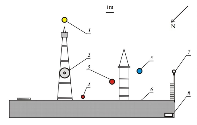
F i g.  1. Layout of the basic measuring systems at the oceanographic platform during the experiments in May – June, 2021: 1 – DVS-6000 acoustic Doppler profiler; 2 – Sigma-1 measuring system; 3 –Vostok-M current velocity meter; 4 – MHI-1308 current meters (4 pcs.); 5 – Workhorse Monitor acoustic Doppler profiler; 6 – oceanographic platform; 7 – string wave recorder; 8 – meteorological system

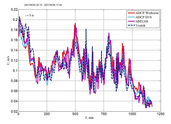
F i g.  2. Mean current velocity module based on measurements by various instruments at the 5 m depth in the area of the oceanographic platform on June 5–6, 2021. The data are reduced to a resolution of 5 min

The results of measurements obtained using different devices were subjected to preliminary processing and primary analysis. This process entailed the removal of faulty sections and implausible values. The sections of records selected for analysis were synchronized and reduced to the same level of discretization for joint processing. Figure 2 shows an example of synchronized and reduced to a single scale data on the current velocity module obtained by measuring simultaneously using different devices (acoustic and spinner) at different points. The averaged data analysis showed that the difference in the values of the current velocity module obtained from measurements conducted using acoustic complexes does not exceed 5%.

In addition to spectral and structural analysis of the measured values, wavelet analysis was used for more accurate identification of synchronous (asynchronous) variability in the current field and coherent structures. Specifically, wavelet analysis permits to identify the energy distribution of the measured values by scale and track its evolution [11]. The continuous wavelet transformation was used

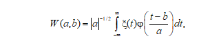
where W denotes the wavelet coefficients, a is the wavelet transformation scale, b indicates the time shift, ξ is the initial signal, φ is the mother wavelet, and t is the time. The Morlet wavelet was predominantly used as the mother wavelet:

The global energy spectrum in wavelet analysis is an analogue of the power spectrum in harmonic analysis. It is generally accepted that this technique reliably reveals spectral peaks; however, it is inferior to the Fourier transform in terms of spectral resolution. The global spectrum was calculated using the following formula:

where n denotes the number of readings in a row.

Basic relationships

The representation of turbulent flows as a set of eddies resulting from the successive decay of large ones into smaller ones, which in turn decay down to the smallest ones, dissipating into heat, has been confirmed in numerous experimental works. One of the most important theoretical assumptions in describing turbulence is A.N. Kolmogorov’s hypothesis on the inertial interval existence in the turbulence spectrum [12]. He demonstrated that the structural function of velocity fluctuations is described by the universal dependence D ~ l^2/3, where l denotes the distance between two measurement points. This dependency is independent of the selection of the origin of coordinates, owing to the statistical homogeneity of velocity fluctuations, and is not influenced by the direction of the spacing of the points. However, it depends on the l value, which is the result of the statistical isotropy of turbulence. For the velocity vector components directed along l (longitudinal structural function),

 .                                    

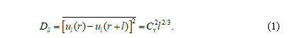
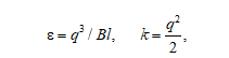
Here,   is the structural parameter characterizing the transformation rate of eddy energy per unit mass. The temperature structural parameter (often referred to as a “structural feature”)   is calculated in a similar way based on the temperature difference at two points or the structural parameter of the refractive index in the atmosphere   [13]. The calculation of structural functions and determination of structural parameters enables the assessment of the turbulence intensity level caused by the energy influx from local and coherent eddies in sea currents. According to Kolmogorov’s theory, the structural parameter is associated with the dissipation rate of turbulent energy, and in the inertial range of the turbulence spectrum  , where c is a constant 

Taking into account Taylor’s "frozen turbulence" hypothesis, the structure function is also calculated from measurements at a specific point, thereby introducing the τ time shift:

The presence of structures in a turbulent flow is evidenced by a noticeable increase in the structural parameter when measured at fixed points. The scale of such eddy formations can be determined from the structural parameter spectrum.

In order to calculate the turbulence intensity and its change with depth in the near-surface layer of the sea, a non-stationary model has been developed [14]. This model is based on the equations of the balance of momentum and turbulent kinetic energy. However, as noted earlier [7, 14], there is a considerable discrepancy between the calculations and experimental data at low winds and slight waves in almost all of the models. In addition, the turbulence generation in the mean transport current is not considered.

In order to account for the impact of coherent structures and the transformation of kinetic energy of the current into turbulence due to local velocity shifts, this paper proposes to introduce an additional term  into the turbulent kinetic energy balance equation. This term describes turbulence generation by these eddy formations. In this form (variation in the structural function over time), the term is expressed in terms of the correspondence to the dimension (m²/s³). The physical meaning of this term is the description of the energy influx to turbulence in the turbulent energy balance equation due to inhomogeneity of the current.

The system of initial equations is expressed as follows:

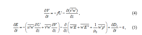
where U and V are the average horizontal velocity components along the x and y axes, respectively; f is the Coriolis parameter;  are the fluctuating velocity components;  is the turbulent kinetic energy; E^w is the energy of surface waves; are the pressure fluctuations; and ε is the dissipation rate. The system is closed through the relations linking the turbulent momentum flows with the turbulent viscosity coefficient:

where ν_t is the turbulent viscosity coefficient; S_m is a constant; l is the turbulent length scale; and ε is the dissipation rate. The l scale depends on the depth as  z is the depth; z_b is the reciprocal wave number of the shortest breaking waves [6]; κ is the von Kármán̰ constant; and the B constant = 16.6.

The initial and boundary conditions, as well as the solution method, remain the same as in [14]. At the upper boundary,

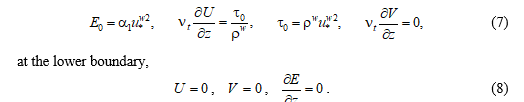
The D_ll structural function in the model is parameterized by a conventional harmonic function that incorporates empirical data. The written system of equations (3)–(8) was solved numerically by the sweep method.

Results

Relatively large coherent structures in the near-surface layer are observed in the energy turbulence spectra. An example of the Fourier spectrum of the root-mean-square velocity fluctuations  averaged over 5 min is shown in Fig. 3. The initial data were obtained at 100 Hz discreteness and then processed with a high-pass filter with a threshold of 1 Hz to remove fluctuations associated with surface waves. The spectra were constructed using the Welch method, where the time series is divided into overlapping segments, multiplied by the Hann time window, Fourier transformed, and then the spectral functions are averaged over all segments.

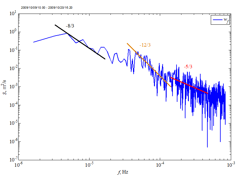
F i g.  3. Spectrum of filtered root-mean-square velocity fluctuations with 5-min averaging in the area of the oceanographic platform based on the measurement data obtained on October 9–20, 2009

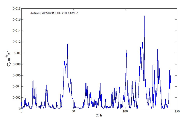
F i g.  4. Longitudinal structural parameter of current velocity fluctuations with 10-min averaging at the 5 m depth in the area of the oceanographic platform on June 1–6, 2021

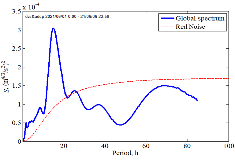
F i g.  5. Global spectrum of structural parameter for June 1–6, 2021

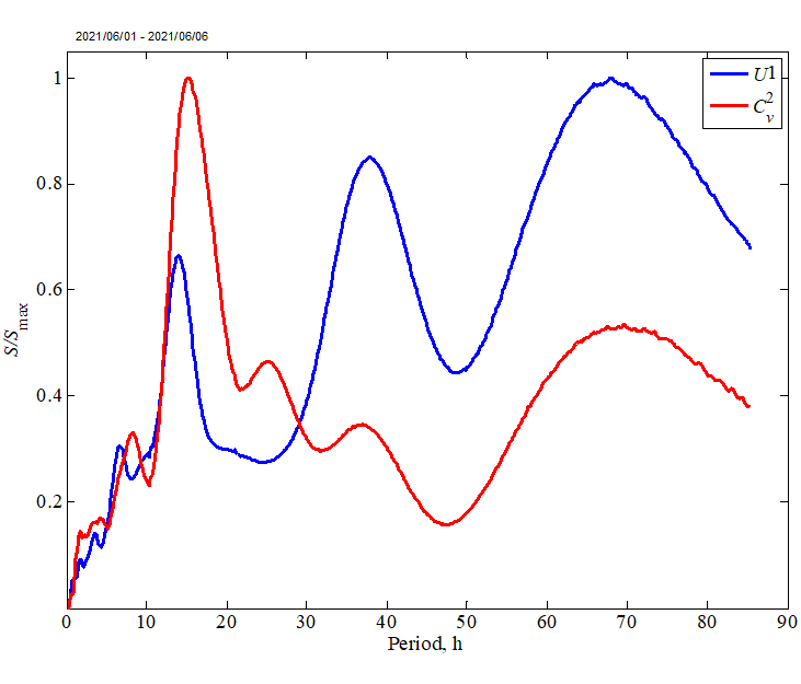
F i g.  6. Normalized global spectra of the current velocity module and structural parameter for June 1–6, 2021

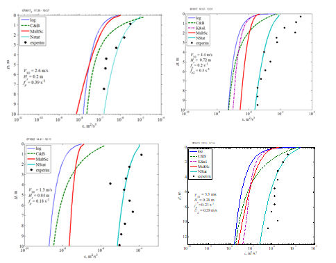
F i g.  7. Model and experimental values of the turbulent energy dissipation rate at low wind. Designations: log is wall turbulence model [4], C&B is model [5], K&al. is model [6]; MultSc is multiscale model [7]; NStat is improved non-stationary model, points are experimental data, V₁₀ is wind speed at the 10 m height, H_S is height of significant waves, f_p is frequency of wave spectral peak, U_d – current velocity

As illustrated in the above figure, the spectrum exhibits a complex shape with various slopes across different ranges. Studies of atmospheric turbulence [13, 15] have demonstrated that coherent turbulence differs from Kolmogorov turbulence by a faster decrease in the spectrum (sections with −8/3 and −12/3 slope), i.e., the presence of such sections in our data indicates the existence of coherent structures.

The principal data array selected for the analysis of synchronous measurements of horizontal current velocity at spaced points and the calculation of structural functions was obtained during the active operational period (01 June 2021 – 06 June 2021) by the DVS-6000 and WorkНorse Monitor complexes (3 and 8 in Fig. 1). A fragment of the records is presented above in Fig. 2. The structural functions were calculated using relations (1) and (2), with the time shift varying from 5 min to 1 h in the latter case. The variability of the  longitudinal structural parameter for the specified period is shown in Fig. 4, and the global spectrum calculated using wavelet analysis is shown in Fig. 5.

Figure 5 shows a clearly expressed maximum in the spectrum at a period of ~ 15 h. This indicates that such structures predominate over a time span of several days. However, when examining shorter intervals, particularly intra-day fluctuations in the intensity of velocity fluctuations, scales with the 1.5- and 3.5-hour periods are clearly visible. It is noteworthy that maxima exceeding the “red noise” level are considered significant in the global spectrum. The current velocity spectrum differs from the spectrum of the structural parameter. As illustrated in Fig. 6, which shows the  global spectrum normalized to its maximum value and the current velocity spectrum calculated from the velocity modulus values, the contribution of currents to turbulence on larger time scales (peaks at ~ 40 and ~ 70 h) is significantly lower than on the 15-hour scale. This is evident from the spectral function level.

The MHI Turbulence Department staff has been conducting experimental observations on the oceanographic platform for a number of years, thus accumulating extensive arrays of data on the turbulent regime of the near-surface layer under various hydrometeorological conditions. The data, which include measurements of the vertical distribution of the turbulent energy dissipation rate, provide a valuable opportunity to verify various models across a range of wind speeds and wave types. As previously mentioned, a notable shortcoming in the modeling of vertical turbulent exchange in the near-surface layer is the discrepancy between calculated and measured values of the dissipation rate at weak winds. A comparison of calculations using the improved model and natural data demonstrated that this issue is largely solved by the proposed method of incorporating additional turbulization of the layer using the structural function.

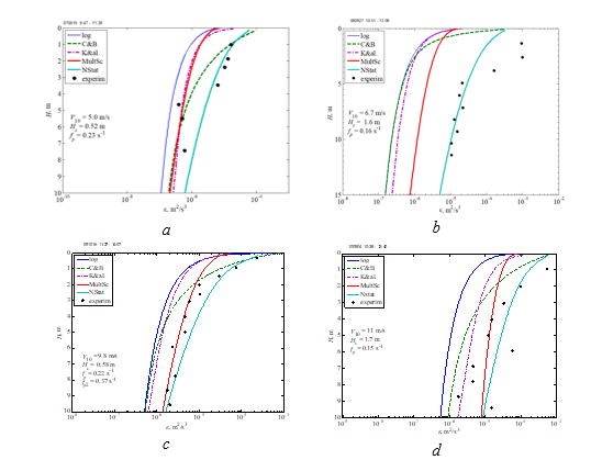
F i g.  8. Model and experimental values of the rate of turbulent energy dissipation at moderate (a, b) and strong (c, d) winds. The designations are the same as in Fig. 7

Figure 7 shows experimental data on the dissipation rate for weak winds along with the results of calculations using various models, including the improved non-stationary model discussed in this paper. A concise overview of the models used for comparison is provided in the Appendix. The figures indicate that the incorporation of an additional source of turbulence, represented by the structure function, significantly improves the agreement between the calculations and in situ measurements. Figure 8 showcases examples of calculations and experimental data for moderate and high winds. In the interest of illustration, preference was given to cases where other models did not align well with the experiments. The agreement between the data of the proposed model and the measurement results under such conditions is also quite satisfactory.

Discussion

According to modern concepts, in turbulent shear flows, the transfer of momentum, energy, and other quantities are predominantly determined by large-scale eddy motion rather than by chaotic small-scale motion. Large formations that emerge in turbulent flows are classified as coherent structures, also referred to as deterministic. According to the definition outlined in the work [16, p. 307], “A coherent structure is a connected turbulent fluid mass with instantaneously phase-correlated vorticity over its spatial extent”. The necessity of parameterizing these structures is justified by the fact that they are able to transfer up to 80% of the total energy of a turbulent current . In experimental data, it is quite difficult to differentiate between coherent and incoherent turbulence, since small-scale turbulence (by Kolmogorov) is also present in the coherent structures. The spectrum shown above (Fig. 3) contains sections that quite accurately correspond to the results of work [15]. Our measurements confirm the complex nature of the turbulent current and the presence of coherent structures within the studied layer. Consequently, the description of turbulent exchange requires additional consideration of this phenomenon. In our estimation, the calculated spectral function provides a reasonably objective characterization of the intensity of turbulence caused by local instabilities in sea currents within the coastal zone.

As illustrated in Fig. 5, structures with specific scales can dominate under certain conditions, thereby enabling the utilization of a model representation of the structural function with a relatively simple dependence at this stage. In this paper, the influence of coherent structures on the turbulence generation is parameterized by a harmonic function with an amplitude and period determined from the experimental values of the longitudinal structural function (Fig. 4). The current is assumed to be uniform along the vertical. The origin and evolution of such structures in the experimental zone require further study. However, it is highly probable that the formation of eddies in the coastal zone of Crimea is similar to the scheme proposed in [17]. Based on our estimates, the spatial scales of eddy formations that significantly affect the generation of turbulence range from several hundred meters to 4–6 km.

As previously stated, the prevalent models for describing vertical turbulent exchange in the upper boundary layer of the sea diverge greatly from observational data in weak and strong winds. Conversely, in moderate winds the models work quite satisfactorily. In our experiments with low winds the discrepancies between the calculation results obtained from different models and the measurement data could reach two orders of magnitude or more [7]. The implementation of the enhanced non-stationary model has improved the agreement between the model data and the experimental results under such weather conditions (Fig. 7).

Importantly, the experimental data presented were collected in different years and seasons, but in the overwhelming majority of experiments the discrepancies between these data and the model data were insignificant. For moderate and strong winds, the model also agrees well with the field measurements (see Fig. 8), and the model constant for the structural function is found to be quite universal, and the model functions well in about 80% of the cases considered. The model values are overestimated at low current velocities of 0.02–0.07 m/s, and underestimated in some cases under storm conditions. The reasons for the discrepancy require a separate analysis of the whole complex of hydrological and meteorological conditions. Thus, it can be tentatively concluded that the influence of coherent structures in the layer turbulence becomes predominant at weak winds, while at moderate and storm winds, their relative contribution to the generation of turbulence in the uppermost layer of the sea decreases.

Conclusion

Insufficient description of the complex exchange processes in the upper boundary layer of the sea gives rise to inaccuracies in forecasting such critical parameters as the mixed layer depth and the ocean surface temperature. In the climate models currently in use, a limited number of turbulence generation mechanisms are considered. These mechanisms determine the intensity of vertical mixing, which often leads to significant differences between the results of calculations and measurement data.

In this paper, an improved approach to vertical exchange description in the near-surface layer of the sea is proposed. This approach involves the incorporation of a term into the turbulent energy balance equation, which describes the generation of turbulence by coherent structures formed in the mean current. The physical substantiation of this approach is rooted in the idea of turbulence generation by local instabilities in the fluid flow at high Reynolds numbers and the shear effects on relatively large-scale eddy structures. The implementation of the structural function concept as a characteristic of the transformation of current energy into turbulence has yielded a highly encouraging result, significantly improving the agreement between the outcomes of calculations and experiments across a broad spectrum of hydrometeorological conditions. The quantitative assessment of the structural function and the structural parameter is founded on the synchronous measurement of current velocity using acoustic meters at horizontally spaced locations. The global spectrum of the structural parameter calculated using wavelet analysis revealed a dominant period of turbulence generation intensity fluctuations. This fluctuation period is apparently associated with the existence of coherent structures of the corresponding scale in coastal sea currents. The experimental data on the temporal variability of the structural function are parameterized by a harmonic function built into the model.

The proposed model was used to conduct calculations, which indicated a significant improvement in the correlation between the calculated results and the experimental data at low winds. The generation of turbulence by the current velocity shift and surface waves is negligible at these wind speeds. Additionally, the model demonstrated a strong agreement with in situ data at moderate and high winds.

Appendix

Turbulence models used for comparison

with the non-stationary model proposed

1. In the model proposed in [4], the assumption is made that turbulence under the ocean surface is similar to turbulence near a solid wall. The rate of turbulent energy dissipation in this case is calculated according to the following formula:

where  is the friction velocity in water; κ is the von Kármán constant; z is the depth. However, as previously mentioned in [4], the application of such an analogy requires the precise selection of the zero surface to filter out small irregular waves. Additionally, the correct averaging of the measured values is essential to obtain the structure of the mean current, similar to the turbulent boundary layer near a flat plate. This model is frequently called logarithmic, according to the velocity change law in a turbulent flow near a solid boundary.

2. One of the most well-known models of turbulence in the near-surface layer was developed in [5], where Prandtl’s hypothesis on the mixing path is used to close the system of equations. This model demonstrates strong agreement with both natural and laboratory experiments [18, 19], and the results are found to be significantly influenced by the value of the z₀ roughness parameter and the choice of the l turbulence scale. The layer near the surface with an increased dissipation rate was interpreted as a consequence of the turbulent energy flow from waves through the surface.

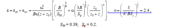
In this model, the dissipation rate and kinetic energy of turbulence are defined as follows:

where q is the rate scale; l is the length scale; B = 16.6 is a constant; l = κ (z + z₀), z is the depth, z₀ is the roughness parameter in water, κ is the von Kármán constant. The model yields both asymptotic analytical and numerical solutions. The dissipation rate is analytically expressed as follows:

To date, this model is the most widely used to describe turbulence near the sea surface and to compare with field and laboratory experiments.

3. In the Kudryavtsev et al. model [6], the velocity shift and wave breaking, including microbreaks, are identified as sources of turbulent energy in the near-surface layer of the sea. Breaking is considered as a volumetric source of energy and momentum, depending on the spectral composition of surface waves. The equation of turbulent energy balance is proposed to be neglected in this model, in contrast to the model from [5]. The z₀ roughness parameter in the surface layer is not included in this model. Numerical calculations using it showed quite satisfactory agreement with the experimental results from [20].

4. The multiscale turbulence model developed in [7] is based on the division of the turbulence spectrum into sections, where turbulence is generated by different mechanisms. For each section, a corresponding system of equations is compiled based on the k-ε model. The turbulence sources are the shift in the drift current velocity, nonlinear effects of surface waves and their breaking. Original parameterizations are proposed for the last two generation mechanisms, and the existence of turbulent diffusion of wave kinetic energy is also estimated. The model demonstrates good agreement across a broad spectrum of hydrometeorological conditions, both in terms of its own natural data and that of other researchers. Notably, the advantages of this model become particularly evident in storm conditions, setting it apart from other similar models.

1. Belcher, S.E., Grant, A.L., Hanley, K.E., Fox-Kemper, B., Van Roekel, L., Sullivan, P.P., Large, W.G., Brown, A., Hines, A. [еt al.], 2012. A Global Perspective on Langmuir Turbulence in the Ocean Surface Boundary Layer. Geophysical Research Letters, 39(18), L18605. https://doi.org/10.1029/2012GL052932

2. Sullivan, P.P. and McWilliams, J.C., 2010. Dynamics of Winds and Currents Coupled to Surface Waves. Annual Review of Fluid Mechanics, 42, pp. 19-42. https://doi.org/10.1146/annurev-fluid-121108-145541

3. Csanady, G.T., 1984. The Free Surface Turbulent Shear Layer. Journal of Physical Oceanography, 14(2), pp. 402-411. https://doi.org/10.1175/1520-0485(1984)014<0402:TFSTSL>2.0.CO;2

4. Benilov, A.Yu. and Ly, L.N., 2002. Modelling of Surface Waves Breaking Effects in the Ocean Upper Layer. Mathematical and Computer Modelling, 35(1-2), pp. 191-213. https://doi.org/10.1016/S0895-7177(01)00159-5

5. Craig, P.D. and Banner, M.L., 1994. Modelling of Wave-Enhanced Turbulence in the Ocean Surface Layer. Journal of Physical Oceanography, 24(12), pp. 2546-2559. https://doi.org/10.1175/1520-0485(1994)024<2546:MWETIT>2.0.CO;2

6. Kudryavtsev, V., Shrira, V., Dulov, V. and Malinovsky, V., 2008. On the Vertical Structure of Wind-Driven Sea Currents. Journal of Physical Oceanography, 38(10), pp. 2121-2144. https://doi.org/10.1175/2008JPO3883.1

7. Chukharev, A.M., 2013. Multitime Scale Model of Turbulence in the Sea Surface Layer. Izvestiya, Atmospheric and Oceanic Physics, 49(4), pp. 439-449. https://doi.org/10.1134/S0001433813040026

8. Pearson, B.C., Grant, A.L.M., Polton, J.A. and Belcher, S.E., 2015. Langmuir Turbulence and Surface Heating in the Ocean Surface Boundary Layer. Journal of Physical Oceanography, 45(12), pp. 2897-2911. https://doi.org/10.1175/JPO-D-15-0018.1

9. Pearson, J., Fox-Kemper, B., Pearson, B., Chang, H., Haus, B.K., Horstmann, J., Huntley, H.S., Kirwan, A.D., Lund, B. [et al.], 2020. Biases in Structure Functions from Observations of Submesoscale Flows. Journal of Geophysical Research: Oceans, 125(6), e2019JC015769. https://doi.org/10.1029/2019JC015769

10. Samodurov, A.S., Dykman, V.Z., Barabash, V.A., Efremov, O.I., Zubov, A.G., Pavlenko, O.I. and Chukharev, A.M., 2005. “Sigma-1” Measuring Complex for the Investigation of Small-Scale Characteristics of Hydrophysical Fields in the Upper Layer of the Sea. Physical Oceanography, 15(5), pp. 311-322. https://doi.org/10.1007/s11110-006-0005-1

11. Astaf’eva, N.M., 1996. Wavelet Analysis: Basic Theory and Some Applications. Advances in Physical Sciences, 39(11), pp. 1085-1108. https://doi.org/10.1070/PU1996v039n11ABEH000177

12. Kolmogorov, A.N., 1968. Local Structure of the Turbulence in an Incompressible Viscous Fluid at Very High Reynolds Numbers. Soviet Physics Uspekhi, 10(6), pp. 734-736. https://doi.org/10.1070/PU1968v010n06ABEH003710

13. Nosov, V.V., Kovadlo, P.G., Lukin, V.P. and Torgaev, A.V., 2012. Atmospheric Coherent Turbulence. Atmospheric and Oceanic Optics, 26(3), pp. 201-206. https://doi.org/10.1134/S1024856013030123

14. Chukharev, A.M. and Pavlov, M.I., 2024. Turbulent Exchange in Unsteady Air–Sea Interaction at Small and Submesoscales. Izvestiya, Atmospheric and Oceanic Physics, 60(1), pp. 87-94. https://doi.org/10.1134/S0001433824700105

15. Lukin, V.P., Nosov, E.V., Nosov, V.V. and Torgaev, A.V., 2016. Causes of Non-Kolmogorov Turbulence Manifestation in the Atmosphere. Applied Optics, 55(12), pp. B163-B168. https://doi.org/10.1364/AO.55.00B163

16. Hussain, A.K.M.F., 1986. Coherent Structures and Turbulence. Journal of Fluid Mechanics, 173, pp. 303-356. https://doi.org/10.1017/S0022112086001192

17. Zatsepin, A.G., Piotukh, V.B., Korzh, A.O., Kukleva, O.N. and Soloviev, D.M., 2012. Variability of Currents in the Coastal Zone of the Black Sea from Long-Term Measurements with a Bottom Mounted ADCP. Oceanology, 52(5), pp. 579-592. https://doi.org/10.1134/S0001437012050177