


N.N. Zubov’s State Oceanographic Institute
Russian Federation
Russian Federation
N.N. Zubov’s State Oceanographic Institute
Russian Federation
N.N. Zubov’s State Oceanographic Institute
Russian Federation
Purpose. The purpose of the work consists in studying the structure and flow routes of the transformed North Sea waters in the Baltic Sea during the formation and spread of the Major Baltic inflow in December 2014 using numerical modeling. Methods and Results. To achieve the stated aim, a three-dimensional baroclinic hydrodynamic model of the North and Baltic seas with a spherical grid area detailed in the Danish straits has been developed based on the INMOM model. Within the framework of the performed numerical experiment, the oceanological characteristic fields were assessed in the system of two seas for the period from 1 January 2014 to 31 December 2015. Comparison of the model-derived salinity and sea current characteristic values with those measured at the Darss Sill and Arkona stations as well as with the BSPAF regional reanalysis data has shown that in general, the INMOM model reproduces changes both in salinity and characteristics of the average currents better than the reanalysis data. The features of vertical variability of salinity and sea currents in the Danish straits during the Major Baltic inflow formation are described based on the modeling results. The daily average and total volumes of water transported in the Sound, Great Belt and Little Belt straits during the main period of the Major inflow are estimated. The features of distribution of the near-bottom salinity fields during different periods of its formation are described. The Lagrangian modeling made it possible to describe the ways in which the waters of the Major Baltic inflow spread. Conclusions. The estimates of water exchange obtained due to the INMOM model indicate that during the main period of the Major Baltic inflow (December 2014), a total of 241.4 km3 of the Kattegat waters passed through the Danish straits. The inflow largest part, 170.9 km3, spread through the Great Belt Strait, while only 68.9 km3 passed through the Sound Strait. The effect of the Small Belt Strait on water transport during the Major Baltic inflow was very insignificant – only 1.6 km3. The study of distribution routes of the transformed North Sea waters over the Baltic Sea after the end of the Major Baltic inflow shows that having passed the Danish straits, its waters spread in a wide flow to the Southwestern Baltic, then penetrate to the Gulf of Gdansk, move further along a cyclonic trajectory through the deep-sea areas of the eastern and northern parts of the Gotland Basin without entering the Gulf of Finland and reach the Landsort Deep in the western part of the Gotland basin by the end of December 2015.
hydrodynamic modeling, INMOM, Baltic Sea, North Sea, Danish straits, Major Baltic inflow, salinity of the Baltic Sea, currents of the Baltic Sea, regional reanalysis of hydrophysical fields, water exchange, water salinity, sea level, stratification of waters, Lagrangian modeling
Introduction
Major Baltic inflows (MBIs) represent the irregular introduction of extremely large volumes of the North Sea waters, from 90 to 258 km3, into the Baltic Sea, lasting 6–29 days, which penetrate into the deep-water areas of the Baltic Proper (Fig. 1), exerting a beneficial effect on the ecological state of this sea [1–7]. Weak inflows of the North Sea waters of 10–20 km3 in volume appear constantly but the penetration of these waters into the Baltic is most often limited to the Arkona Basin (Fig. 1). MBIs are a relatively rare phenomenon observed until the early 1980s from 1–2 times a year to once every few years [4]. Spreading far into the open part of the Baltic Sea, highly saline and oxygen-rich waters of large inflows renew the bottom and deep-water Baltic masses exposed to hypoxic conditions [2, 4, 8]. Observations show that after 1983, the number of MBIs decreased significantly and the interval (stagnation period [8]) between them increased greatly and amounted to 10–11 years [4, 6, 7–9]. Physical mechanisms for the increase in stagnation periods remain unexplored to date. The last major inflow occurred in December 2014 [5], after which no new MBIs have been described in the scientific literature.
MBIs can be considered as an extreme water exchange component between the North and Baltic seas. For example, according to K. Wyrtki [10] and H. Fischer and W. Matthäus [3], about 200–225 km3 of the Kattegat waters passed through the Danish straits during the MBI in November – December 1951, which amounted to approximately 40% of the annual norm.
The accumulated information on the variability of hydrometeorological processes during MBI allowed scientists to identify four periods in the process of its formation: outflow period, precursory period, main inflow period and post inflow period [4, 5, 8].
The outflow period starts when eastern winds blow over Northwestern Europe, which contributes to the water outflow from the Baltic into the North Sea and its level decrease. This period is very important for the future formation of MBIs since the longer and more intense the water outflow from the Baltic is, the more its level will decrease and the greater the level gradient between the Kattegat and the Southwestern Baltic will form before the beginning of MBIs. The intensity of MBIs depends largely on this gradient [4, 5, 8].
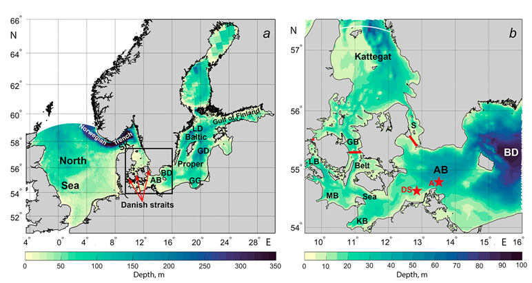
F i g. 1. Bathymetry of the North and Baltic seas (black square indicates the area of the Southwestern Baltic and the Kattegat) (a), enlarged image of the selected area (b). Designations: asterisks show location of the Darss Sill (DS) and Arkona (A) automatic stations; AB is the Arkona Basin, BD is the Bornholm Deep, GD is the Gotland Deep, LD is the Landsort Deep, LB is the Little Belt Strait, GB is the Great Belt Strait; S is the Sound Strait, SK is the Skagerrak, MB is Mecklenburg Bay, KB is Kiel Bay, GG is the Gulf of Gdansk
In the precursory period, the synoptic situation changes: the east wind weakens and begins to change its direction to the west one. This leads to the sea level elevation in the Kattegat, gradually approaching the level in the Southwestern Baltic [4, 5, 9].
The main inflow period occurs when the North Sea level elevation, which began in the previous period, reaches a critical value, at which the level gradient becomes directed from the Kattegat to the Southwestern Baltic and continues to grow under the influence of strong west winds, the duration of which reaches 2–3 weeks. At this time, the difference in level between the Kattegat Strait and the Southwestern Baltic (Fig. 1, b) can reach 1.0–1.7 m [11]. As a result, large masses of the highly saline and oxygen-rich Kattegat waters enter the Baltic Sea, which, in turn, leads to a further decrease in the North Sea level and an increase in the Baltic Sea [4, 5, 8].
The post inflow period begins when the west winds weaken and the North Sea waters cease to accumulate in the Danish straits. Since the Baltic Sea level is elevated relative to the North Sea level, the water outflow from the Baltic Sea begins and its level drops to a level close to its average value [4, 7, 8].
Mathematical modeling of water exchange and oceanographic conditions in the North and Baltic Seas is a complex task for two main reasons. Firstly, the oceanographic regimes of these seas are very different. The North Sea is a shallow (except for the Norwegian Trench) (Fig. 1, a), weakly stratified marine basin with intense tidal dynamics and vertical mixing, relatively freely communicating with the ocean, so its salinity is close to oceanic. On the contrary, the Baltic Sea is an almost completely closed brackish marine basin with very weak tidal dynamics and sharp stratification, limiting vertical mixing between surface and deep-water masses. Secondly, due to the narrowness and shallowness of the Danish straits connecting the North and Baltic Seas (the Sound, the Great Belt and the Little Belt) (Fig. 1, b), which have a complex morphometry of the coastline and bottom topography. The minimum width of the Sound is less than 5 km and its smallest depth is 8 m; for the Great Belt Strait, these parameters are 3.7 km and more than 20 m; for the Little Belt Strait, they are 0.8 km and 12 m, respectively [8, 12, 13].
Such characteristics of the Danish straits require the use of a grid domain with cells of significantly smaller dimensions than the smallest width of the straits in numerical modeling for correct water flow simulation in these straits as well as the features of stratification and current structure. Processing power of modern computers does not make it possible to use uniform grids with such a high spatial resolution for modeling not only the combined water area of the North and Baltic seas, but also the Baltic Sea alone. To solve this problem, scientists expanded the Danish straits artificially when modeling the oceanographic conditions of the Baltic Sea, adjusting their width to the spatial resolution of the grid domain used in the model [14–16]. Such a procedure, with an unchanged depth, led to a change in the cross-sectional area of the straits. Therefore, the depth of the straits was reduced to maintain the cross-sectional area. Both changes in the morphometry of the straits lead to changes in stratification, current structure and salt transport volume in the Danish straits [12].
An important length scale that should be taken into account when modeling oceanographic fields for correct resolution of mesoscale eddies, upwellings [17] and structure of narrow jets caused by the dynamics of gravity currents in the Southwestern Baltic [18, 19] is the baroclinic Rossby radius of deformation. According to estimates by various researchers, its largest values (7–9 km) were observed in the Bornholm Basin and deep-water areas of the Baltic Proper, with the smallest (1–2 km) ones in the sea shallow areas with depths less than 50 m [20–23]. In this regard, models with nested grids have been used to improve the spatial resolution in numerical experiments. For example, in [12], the model domain with a nested uniform grid had a spatial resolution of 900 m and included the waters of the Kattegat, the Danish straits and the Arkona and Bornholm basins of the Baltic (Fig. 1, b). One of the liquid boundaries of the model was located in the north of the Kattegat and the other one – in the east of the Bornholm Basin [12]. However, such models do not allow studying the propagation routes of the MBI waters in other Baltic Sea areas.
In our opinion, models with unstructured grids with the highest condensation (detailing) in the area of the Danish straits are more promising for the MBI studying, which allows for a more accurate description of the structure of currents, stratification of water masses and salt transport through narrow and shallow straits. In [24], a joint model of the North and Baltic Seas with a mixed triangular-quadrangular unstructured grid was used, which made it possible to achieve a nominal spatial resolution of 200 m in the Danish straits. Comparison of the modeling results with data from tide gauge measurements of sea level and measurements of temperature and salinity at the Fehmarn Belt and Arkona stationary stations showed good agreement overall, although in some areas of the compared series, the discrepancies between the measured and calculated values reached 30–50 cm for sea level, 3–5°C for temperature and 2–3‰ for salinity [24].
The main purpose of the paper is to estimate the capabilities of numerical hydrodynamic modeling of MBIs using a 3D baroclinic model of the North and Baltic Seas, which has a spherical grid area with detailing in the Danish straits, and, based on the modeling results, to study the structure and propagation routes of the transformed North Sea water flows in the Baltic Sea after the MBI in December 2014.
Data and methods
Model description
The Institute Numerical Mathematics Ocean Model (INMOM) of ocean and sea circulation developed at Marchuk Institute of Numerical Mathematics of RAS [25, 26] was chosen as the basic model to describe oceanological processes in the Baltic and North Sea systems during the 2014 MBI.
The INMOM is based on a complete system of nonlinear primitive equations of ocean hydrodynamics in spherical coordinates in the hydrostatic and Boussinesq approximations. Dimensionless quantity  is used as a vertical coordinate, where z is usual vertical coordinate;
  is deviation of the sea level from the undisturbed surface as a function of longitude λ, latitude φ and time t;
  is sea depth. The number of vertical sigma layers in the model is 20.
The predictive variables of the model are horizontal components of the velocity vector, potential temperature, salinity and ocean level deviation from the undisturbed surface. To calculate the density, a specially designed for numerical models [27] equation of state that takes into account the compressibility of seawater is used.
The coefficients of vertical turbulent diffusion and viscosity were selected according to the Pacanowski – Philander parameterization [28]. The coefficient of turbulent diffusion varied from 1 to 50 cm2/s and the coefficient of turbulent viscosity varied from 1 to 250 cm2/s. Horizontal turbulent diffusion and viscosity were described by the usual Laplacian with coefficients  = (3–8)×104 cm2/s. Bottom friction was specified by a quadratic equation with coefficient CD = 2.5×10⁻⁴.
The model includes a sea ice thermodynamics block [29] consisting of three modules. The thermodynamics module describes freezing, ice melting and snowfall. The ice dynamics module calculates its drift velocities. The ice transport module is used to calculate the ice and snow cover evolution due to the drift [30].
The model uses a spherical grid with two poles, one of which is located on the Jutland Peninsula (Denmark) and the other – in the very south of Sweden (Fig. 2). The spatial resolution of the grid area nodes in the area of the Danish straits is about 300–700 m and increases proportionally to 6–12 km with distance from the straits towards the outskirts of two seas.
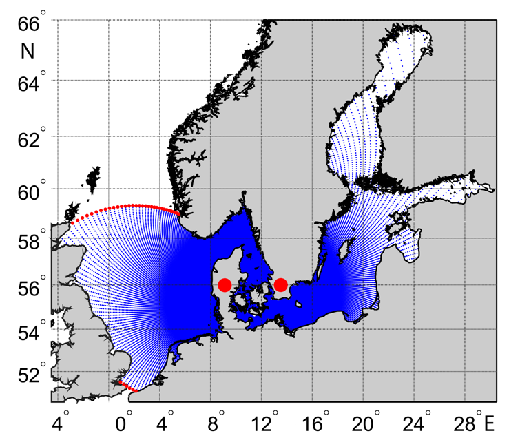
F i g. 2. Grid area of the model. Red dots indicate model liquid boundaries, black circles – grid area poles
For this model version, bathymetry from GEBCO 2015 was combined. When preparing the model bathymetry, depth values were interpolated into grid nodes and smoothed with a Gaussian filter to eliminate their sharp differences, which increases significantly the stability of calculations during modeling.
Initial and boundary conditions
The initial conditions were monthly average water temperature and salinity data for January 2014 with a vertical resolution of 5 m and a spatial resolution of 4.5 × 9 km from the GLORYS12V1 ocean reanalysis (available at: http://marine.copernicus.eu).
For the boundary conditions on the sea surface in the INMOM atmospheric module, such meteorological characteristics as air temperature and humidity at a height of 2 m, pressure at sea level, wind speed at a level of 10 m, incident shortwave and longwave radiation, atmospheric precipitation were specified with a discreteness of 3 hours, a spatial step of 0.25° and duration from January 2014 to December 2015 obtained from the ERA5 reanalysis .
At the liquid boundaries of the North Sea (Fig. 2), the average monthly values of water temperature and salinity observed from January 2014 to December 2015 as well as the amplitudes and phases of the oscillations of the level and currents of eight main tidal harmonics (M2, S2, N2, K2, K1, O1, P1, M4) taken from TPXO9 global tidal model (available at: https://www.tpxo.net/global) were specified.
On the solid sections of the lateral boundary, the heat and salt fluxes were set equal to zero and the no flow and free sliding conditions were used for the current velocity.
Model calculations were carried out from 1 January 2014 to 31 December 2015, with the average results being derived for each hour.
Verification of the model and comparison of the modeling results with the data of regional reanalysis of hydrophysical fields
To verify the model, we used the data from contact measurements of salinity and currents at different horizons of stationary automatic stations Darss Sill and Arkona located in the Southwestern Baltic at 21 and 45 m depths, respectively (Fig. 1, b). Observations of salinity at the Darss Sill station are made at 2, 5, 7, 12, 17 and 19 m horizons and at the Arkona station – 2, 5, 7, 16, 25, 33, 40 and 43 m. Current velocity and direction are measured with Doppler acoustic profilers at these stations.
The INMOM modeling results were compared with instrumental measurements as well as with salinity and current change data obtained using the regional reanalysis of the Baltic Sea Physics Analysis and Forecast (BSPAF) hydrophysical fields based on the numerical implementation of the Nucleus for European Modeling of the Ocean (NEMO) 3.6 hydrodynamic model [31, 32] for the Baltic Sea conditions. This model uses a procedure for contact and satellite information assimilation based on the algorithm of one of the varieties of the Kalman filter (local singular evolutive interpolated Kalman (LSEIK) filter) [33]. Satellite data on surface water temperature provided by the Swedish Meteorological and Hydrological Institute (SMHI) ice service as well as in situ T and S measurements from the ICES database (available at: http://www.ices.dk) were used as assimilated variables in the NEMO 3.6 model. The NEMO 3.6 model used meteorological data computed with the ECMWF ERA5 atmospheric model to set the sea surface boundary conditions. The BSPAF regional marine reanalysis data are daily averaged, they have a horizontal resolution of 3.9 km and 56 vertical horizons (layer thickness varies with depth from 3 to 22 m) and cover the 1993–2022 period.
To compare the salinity changes measured and calculated with the INMOM model and the BSPAF reanalysis data at different depths, mathematical expectations of salinity series ms, their standard deviations (SD) ss, minimum Smin and maximum Smax values and correlation coefficient Rss between the measured and model salinity values were estimated. The accuracy of the salinity values calculated using the INMOM and NEMO 3.6 models (BSPAF reanalysis) was estimated using accuracy criterion Pa, which shows the number of salinity values calculated using the models that fall within range < 0,674s, where s is SD of the salinity values measured at the Darss Sill and Arkona stations.
To compare the measured and model values of currents, the following statistical characteristics of the variability of the velocity and direction of currents were estimated using the vector-algebraic method of analysis of random processes.
1) mathematical expectation of vector process mv (module direction  and direction am);
2) linear invariant of the SD tensor [I1(0)]0,5, where I1(0) = l1(0) + l2(0) is linear invariant of the vector process dispersion tensor determined through the half-lengths of principal axes l1(0) и l2(0) of the dispersion ellipse and orientation a° of its major axis relative to the geographic coordinate system:
where  are dispersions of the vector process components;
3) stability of currents ½ ½, where ½
 ½ is module of the mathematical expectation of a vector process. When r > 1, the intensity of oscillatory motions in the flow prevails over the intensity of the average transfer, i.e. the current is unstable; when r < 1, currents become more stable;
4) two invariants of the normalized cross-correlation tensor function between the currents measured at the Darss Sill station and calculated using the INMOM model and BSPAF data: linear invariant I1VU(t) and rotation indicator DVU(t). Linear invariant I1VU(t) is equal to the trace of the matrix of correlation tensor function KVU(t), two vector processes V(t) and U(t) and characterizes the integral of the intensities of collinear changes in vector processes V(t) and U(t):
KVU(t) =
where t is time shift; v1 is component of vector process V(t) on the parallel; v2 is component of vector process V(t) on the meridian; u1 is component of vector process U(t) on the parallel; u2 is the component of vector process U(t) on the meridian.
Rotation indicator DVU(t) is equal to the difference of the non-diagonal components of the matrix of correlation tensor function KVU(t) and characterizes the integral of orthogonal changes in processes V(t) and U(t); when DVU(t) > 0, process U(t) is rotated on average relative to process V(t) over a given time period clockwise and counterclockwise when DVU(t) < 0.
Then the total correlation coefficient was calculated:
RVU( =
=
In addition, the maximum modules of current velocity  max were estimated.
Flow rates of currents Q through the Danish straits during the 2014 MBI formation were estimated based on the current velocity vectors (V) calculated by the INMOM model at different horizons along three sections crossing the straits (see Fig. 1, b), using the following formula:
where n is number of i-cells on the section; m is number of z-horizons in the given cell;  is meridional component of the current velocity in a grid cell at horizon z; S is cross-sectional area of the cell determined as product of layer thickness (∆z) and distance between adjacent nodes of the grid region of model (
 ), i.e.
  .
.
To study the propagation routes of transformed North Sea waters after the MBI, two methods were used. The first method made it possible to construct two oceanographic sections along a system of interconnected deep-water basins of the marine relief. Their location was determined based on published information on the migration routes of the salty North Sea waters during the MBI in the Baltic Sea [4, 5]. Using the modeling data, diagrams of the temporal variability of salinity in the bottom layer were constructed on these sections. In the second case, the Lagrangian method was used. Its detailed description is given in [34]. Within the framework of this method, 5000 passive markers were placed daily from 1 November to 31 December 2014 on a segment along the boundary passing north of the Danish straits along a line with coordinates 56.6°N, 10.85°E – 56.6°N, 11°E (Fig. 1, b). Based on the current velocity vector fields calculated using the INMOM model, each marker trajectory was calculated for a period of one year (until 31 December 2015).
Lagrangian trajectories were calculated using advection equation
where u and v are angular components of the current velocity calculated using the INMOM model in the penultimate s-layer in depth; φ and λ denote latitude and longitude, respectively. Angular velocities are used to simplify the equation of motion on a sphere. Velocity values inside the grid cells were calculated using bicubic interpolation in space and third-degree Lagrange polynomial interpolation in time. When modeling the Lagrangian trajectories, the coordinates of the passive markers were recorded with the 1 h time resolution.
Results and discussion
Comparison of salinity and current values measured and calculated with the INMOM model and BSPAF reanalysis
Figs. 3 and 4 show changes in salinity values obtained during measurements at different horizons of the Darss Sill and Arkona automatic stations (see Fig. 1, b for the location of stations) based on the INMOM modeling results and the BSPAF regional reanalysis data for 1 November – 31 December 2014. Table 1 shows the statistical estimates of the measured and model salinity values. It is evident that the December 2014 MBI is modeled both by the BSPAF regional reanalysis data and by the INMOM modeling results as an anomalously large increase in salinity from the bottom horizons to the sea surface (Figs. 3 and 4). At the same time, the BSPAF reanalysis data, unlike the INMOM model, did not reproduce two weak inflows of the Kattegat waters that occurred on 22 and 26 November 2014 (Fig. 3). The correlation coefficients (Rss) between the measured and model (INMOM and BSPAF) salinity series at different horizons are high and vary from 0.70 to 0.98 near the Darss Sill station and from 0.67 to 0.98 near the Arkona station (Table 1). This result indicates that the reanalysis data and the INMOM model describe adequately the main features of salinity changes during the MBI in the Southwestern Baltic, although the values of correlation coefficient Rss between the measurement results and the INMOM data for three upper horizons near the Darss Sill station are noticeably higher than those of BSPAF, while they are close for three lower horizons. On the contrary, for the Arkona station area, the Rss values at three upper horizons are lower for INMOM compared to BSPAF and the Rss values at three lower horizons for INMOM are higher than those of BSPAF (Table 1).

F i g. 3. Water salinity at the Darss Sill station based on the measurement (a), BSPAF reanalysis (b) and INMOM modeling (c) data from 1 November to 31 December 2014
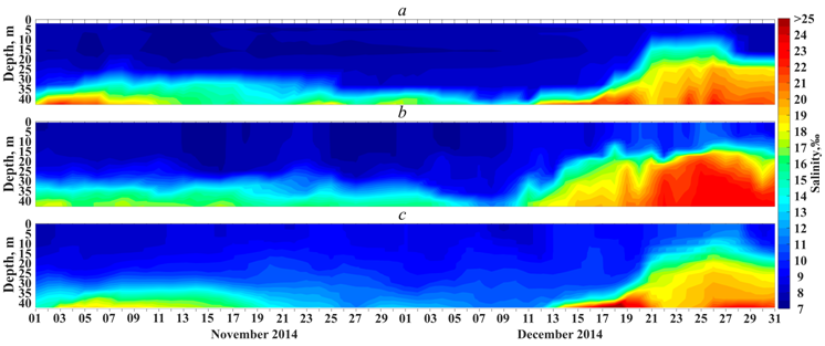
F i g. 4. Water salinity at the Arkona station based on measurement (a), BSPAF reanalysis (b) and INMOM modeling (c) data from 1 November to 31 December 2014
The values of the mathematical expectation of salinity changes during the BSPAF formation and propagation period estimated by INMOM in the Darss Sill station area are overestimated by 9–21% relative to the measured values at almost all horizons and by 4–22% in the area of the Arkona station. The exception is the 40 m horizon where the INMOM results in the Arkona area showed an underestimation of the mathematical expectation of salinity changes by 7% (Table 1). In contrast to the INMOM results, discrepancies between measured and calculated values of the mathematical expectation of salinity changes based on the BSPAF reanalysis data are generally significantly smaller and vary from 0.3 to 7% in the Darss Sill station area and from 2 to 17% near the Arkona station (Table 1). Only at the 25 and 33 m horizons in the Arkona area, the excess of the mathematical expectation values according to the BSPAF data relative to the measurements is noticeably greater than according to the INMOM data (Table 1).
T a b l e 1
Statistical estimates of daily average seawater salinity at different horizons based on the measurements at the Darss Sill (DS) and Arkona (A) stations as well as the INMOM modeling and BSPAF reanalysis data for the period from 1 November to 31 December 2014
|
|
Data source |
Horizon, m |
ms, ‰ |
ss, ‰ |
Smin, ‰ |
Smax, ‰ |
Rss |
Pa, % |
|
|
Darss Sill station |
|
||||||||
|
DS |
2 |
10.93 |
3.37 |
8.07 |
19.21 |
– |
– |
|
|
|
INMOM |
12.10 |
3.57 |
8.68 |
20.51 |
0.90 |
51 |
|
||
|
BSPAF |
10.90 |
4.32 |
7.32 |
20.55 |
0.87 |
16 |
|
||
|
DS |
5 |
11.22 |
3.81 |
8.07 |
20.15 |
– |
– |
|
|
|
INMOM |
12.54 |
3.60 |
9.33 |
20.93 |
0.97 |
56 |
|
||
|
BSPAF |
11.13 |
4.55 |
7.52 |
21.80 |
0.89 |
25 |
|
||
|
DS |
7 |
10.86 |
3.85 |
7.47 |
19.45 |
– |
– |
|
|
|
INMOM |
13.10 |
3.59 |
9.61 |
21.27 |
0.98 |
43 |
|
||
|
BSPAF |
11.61 |
5.00 |
7.67 |
22.43 |
0.88 |
16 |
|
||
|
DS |
12 |
12.28 |
4.42 |
8.05 |
21.26 |
– |
– |
|
|
|
INMOM |
14.52 |
3.55 |
10.12 |
21.54 |
0.89 |
44 |
|
||
|
BSPAF |
12.91 |
5.32 |
7.90 |
23.00 |
0.89 |
18 |
|
||
|
DS |
17 |
14.44 |
4.47 |
8.13 |
21.57 |
– |
– |
|
|
|
INMOM |
15.80 |
3.44 |
11.07 |
21.95 |
0.78 |
44 |
|
||
|
BSPAF |
14.62 |
5.49 |
8.11 |
24.50 |
0.77 |
18 |
|
||
|
DS |
19 |
15.80 |
4.32 |
8.21 |
21.93 |
– |
– |
|
|
|
INMOM |
17.39 |
3.51 |
11.89 |
23.90 |
0.71 |
57 |
|
||
|
BSPAF |
15.49 |
5.74 |
8.11 |
25.33 |
0.70 |
20 |
|
||
|
Arkona station |
|
||||||||
|
A |
2 |
8.16 |
0.52 |
7.58 |
9.71 |
– |
– |
|
|
|
INMOM |
8.98 |
0.85 |
7.63 |
11.41 |
0.78 |
38 |
|
||
|
BSPAF |
8.28 |
1.04 |
7.24 |
11.08 |
0.86 |
7 |
|
||
|
A |
5 |
7.75 |
0.51 |
7.14 |
9.33 |
– |
– |
|
|
|
INMOM |
9.03 |
0.90 |
7.63 |
11.86 |
0.67 |
38 |
|
||
|
BSPAF |
8.29 |
1.05 |
7.32 |
11.11 |
0.81 |
7 |
|
||
|
A |
7 |
7.93 |
0.54 |
7.36 |
9.69 |
– |
– |
|
|
|
INMOM |
9.09 |
0.96 |
7.65 |
12.14 |
0.78 |
38 |
|
||
|
BSPAF |
8.33 |
1.10 |
7.32 |
11.15 |
0.83 |
7 |
|
||
|
A |
16 |
8.39 |
2.34 |
7.14 |
15.59 |
– |
– |
|
|
|
INMOM |
10.2 |
2.10 |
8.35 |
16.86 |
0.83 |
72 |
|
||
|
BSPAF |
9.59 |
3.24 |
7.32 |
19.26 |
0.70 |
26 |
|
||
|
A |
25 |
10.15 |
4.08 |
7.65 |
19.87 |
– |
– |
|
|
|
INMOM |
11.49 |
3.17 |
9.10 |
19.16 |
0.98 |
82 |
|
||
|
BSPAF |
11.84 |
5.01 |
7.48 |
22.51 |
0.89 |
20 |
|
||
|
A |
33 |
12.57 |
4.27 |
7.99 |
20.64 |
– |
– |
|
|
|
INMOM |
13.12 |
3.09 |
10.04 |
19.93 |
0.93 |
77 |
|
||
|
BSPAF |
14.51 |
4.35 |
8.36 |
23.19 |
0.80 |
49 |
|
||
|
A |
40 |
16.56 |
3.15 |
9.09 |
21.98 |
– |
– |
|
|
|
INMOM |
15.42 |
3.46 |
10.84 |
23.06 |
0.86 |
33 |
|
||
|
BSPAF |
16.98 |
3.31 |
10.60 |
23.28 |
0.83 |
49 |
|
||
N o t e: ms is average value; ss is SD; Smin, Smax are minimum and maximum salinity values; Rss is correlation coefficient between the measured and modeled salinity values; Pa is accuracy criterion for the salinity values calculated by the models
Discrepancies between the SD values of salinity according to the INMOM model and results of measurements in the Darss Sill station area in the upper 2–7 m layer are small and do not exceed ±5…7% (Table 1). However, deeper down, the INMOM results show SD values that are underestimated by 19–23%. On the contrary, SD estimates according to the BSPAF reanalysis data show values that are overestimated by 19–33% at all horizons (Table 1).
The estimates of salinity SD measured at the Arkona station at the 2–7 m upper horizons are very small (0.51–0.54‰), which is 6.5–7.5 times less than the estimates of salinity SD based on the measurements at the Darss Sill station (Table 1). At these horizons, SD of salinity obtained from the modeling and reanalysis results shows overestimated values: 0.85–0.96‰ for INMOM and 1.04–1.10‰ for BSPAF. At a depth over 7 m, the estimates of salinity SD based on the measurements at the Arkona station increase significantly (by 4–8 times). Here, in the 16–33 m layer, the estimates of salinity SD obtained from the INMOM modeling results are underestimated by 10–28% relative to the measurement data and only at the bottom horizon of 44 m, they are overestimated by 10% (Table 1). The estimates of salinity SD obtained from the BSPAF reanalysis results are overestimated everywhere at depths from 16 to 40 m. They are overestimated most of all at the 16 m (38%) and 25 m (23%) horizons and not significantly at the 33 m (2%) and 40 m (5%) horizons (Table 1).
Comparison of the measured and model-calculated salinity minimum values shows that according to the INMOM results, they are always greater than their measured values at the Darss Sill and Arkona stations in all cases. Moreover, these discrepancies with the measured values increase from the surface where they do not exceed 1–8% to the bottom horizons where they reach 19–45%.
The discrepancies between the measured and BSPAF reanalysis-calculated salinity minimum values in the areas of the Darss Sill and Arkona stations are noticeably smaller and do not exceed ±9…17% (Table 1).
Comparison of the model-calculated estimates of salinity maxima (Smax) with their measured values at the Darss Sill and Arkona stations during the MBI formation and spread period shows that they exceed the measured values almost in all cases (Table 1). In the Darss Sill station area, the Smax model values based on the INMOM results are 1–9% higher than the measured values while they are significantly higher according to the BSPAF reanalysis data, amounting to 7–16% (Table 1).
For the Arkona station area, the Smax model estimates for INMOM exceed the measured values by 18–27% while those obtained from BSPAF reanalysis data are greater than the measured values by 14–19% (Table 1). At greater depths (16–40 m), discrepancies between the Smax estimates calculated from INMOM and its measured values are noticeably smaller and vary from −4 to +8%. The Smax estimates obtained from BSPAF reanalysis data exceed its measured values by 6–24% (Table 1).
Estimates of the Pa accuracy criterion show that the INMOM model simulates salinity changes in the Southwestern Baltic in general better than the BSPAF reanalysis (Table 1). In the Darss Sill area, 43 to 57% of the INMOM salinity estimates fall within the range of measured values less than 0.674s while only 16 to 25% of the values from the BSPAF reanalysis fall within this range (Table 1). For the Arkona area, the estimates of the Pa accuracy criterion from the INMOM modeling results vary from 33 to 82% while from the BSPAF reanalysis they do not exceed 7–49% (Table 1).
T a b l e 2
Statistical estimates of current velocity variability at different horizons (H) at the Darss Sill station (DS) based on the measurement, BSPAF reanalysis and INMOM modeling data for the period from 1 November to 31 December 2014
|
Data source |
H, m |
cm/s |
/ am, degree |
[I1(0)]0.5, cm/s |
|
|
a°, degree |
RVU ( |
r |
|
|
DS |
2.0 |
3.09 |
337 |
30.04 |
23.26 |
19.00 |
3.18 |
– |
9.7 |
102.7 |
|
BSPAF |
1.5 |
5.73 |
273 |
26.82 |
25.54 |
8.19 |
−0.25 |
0.71 |
4.7 |
59.9 |
|
INMOM |
2.0 |
2.75 |
38 |
20.54 |
19.69 |
5.85 |
8.29 |
0.59 |
7.5 |
37.7 |
|
DS |
5.0 |
3.22 |
346 |
26.93 |
22.51 |
14.79 |
–9.36 |
– |
8.4 |
79.5 |
|
BSPAF |
4.5 |
5.63 |
270 |
26.18 |
24.99 |
7.81 |
–0.79 |
0.67 |
4.6 |
59.1 |
|
INMOM |
5.3 |
2.25 |
42 |
18.14 |
17.58 |
4.50 |
7.44 |
0.55 |
8.1 |
33.6 |
|
DS |
11.0 |
1.31 |
94 |
20.54 |
19.52 |
6.39 |
−19.87 |
– |
15.7 |
55.0 |
|
BSPAF |
10.6 |
3.54 |
245 |
21.79 |
21.28 |
4.66 |
−8.92 |
0.51 |
6.2 |
52.6 |
|
INMOM |
11.2 |
2.72 |
67 |
14.75 |
14.18 |
4.09 |
−2.41 |
0.60 |
5.4 |
27.8 |
|
DS |
14.0 |
2.39 |
83 |
18.67 |
17.59 |
6.27 |
−21.55 |
– |
7.8 |
46.1 |
|
BSPAF |
13.6 |
2.22 |
190 |
19.94 |
19.27 |
5.15 |
−13.50 |
0.61 |
9.0 |
46.6 |
|
INMOM |
14.2 |
3.38 |
76 |
13.77 |
13.02 |
4.47 |
−16.63 |
0.60 |
4.1 |
26.5 |
|
DS |
16.0 |
2.62 |
70 |
17.42 |
16.59 |
5.32 |
−24.98 |
– |
6.6 |
39.8 |
|
BSPAF |
16.8 |
2.73 |
159 |
19.07 |
17.95 |
6.45 |
−18.50 |
0.66 |
7.0 |
38.1 |
|
INMOM |
16.2 |
3.67 |
68 |
13.26 |
12.41 |
4.68 |
−24.57 |
0.66 |
3.6 |
22.5 |


N o t e:  is module of the average value; am is direction of the average value; [I1(0)]0,5 is linear invariant of the SD tensor;
  and
and  are half-lengths of major and minor axes of the SD ellipse; a° is direction of the major axis of SD ellipse; RVU(
 ) is total correlation coefficient; r is current stability indicator;
  max is module of the maximum sea current vector.
Comparison of statistical estimates of current velocities measured at the Darss Sill station and calculated using BSPAF reanalysis data and the INMOM model shows that in the upper 11-meter layer, the  estimates of the mathematical expectation of current velocities obtained using BSPAF reanalysis data are overestimated by 1.8–2.7 times relative to the measured ones while the estimates are close to each other deeper than this layer (Table 2). According to the estimates of am mathematical expectation vector direction, discrepancies between the measured and BSPAF reanalysis values are very large: 64–76° in the upper 5-meter layer, almost opposite at a horizon of about 11 m and reaching 89–107° in deeper layers. In contrast to BSPAF, the INMOM model shows a slight underestimation of by 0.3–1.0 cm/cm in the upper 5-meter layer and their overestimation by 0.99–1.41 cm/s in deeper layers (Table 2). In the am direction, the discrepancies between the measured and calculated estimates using the INMOM model reach 56–61° in the upper 5-meter layer and comparison shows the closeness of the measured and calculated am values deeper than this layer (Table 2).
Estimates of various invariants of the SD tensor of the velocity vectors of the measured and model currents show that in the upper 5-meter layer, the BSPAF results slightly underestimate (by 3–11%) the values of invariant [I1(0)]0,5, which describes the total intensity of current oscillations, and deeper than 5 m, on the contrary, they slightly overestimate it by 6–9%. Comparison of the measured and [I1(0)]0,5 INMOM-modeled estimates shows their significant underestimation (by 24–33%) at all horizons (Table 2). According to instrumental measurements, compression of the SD ellipses of current oscillations in the 2–5 m layer is small while, according to the BSPAF and INMOM model estimates, the minor axes of the SD ellipses in this layer are 3–4 times smaller than the major ones (Table 2). Deeper than this layer, both instrumental measurements and model estimates show a greater degree of compression of the SD ellipses (Table 2).
The directions of the large axes of the SD ellipses of the measured and modeled current oscillations are approximately the same (Table 2).
From the BSPAF reanalysis data and measurement results, correlation coefficients RVU( ) among current oscillations vary from 0,51 to 0,71 and for INMOM, they are 0.55–0.66 (Table 2).
Current stability index r for both measured and model currents at all horizons is significantly greater than 1, which indicates significant instability of the currents during the MBI formation (Table 2).
Comparison of the estimates of the max measured and model currents maxima shows that the INMOM model underestimates their values significantly at all horizons (Table 2). For the BSPAF reanalysis, the same trend is observed only for the 2–5 m layer, and deeper than this layer, the measured and model values of current maxima are comparable (Table 2).
Summarizing the results of the measured and model currents comparison, it can be concluded that the INMOM model reproduces the characteristics of average flows at different horizons during the 2014 MBI formation better and the BSPAF reanalysis data describe the characteristics of oscillatory movements in the deep and bottom layers often more realistically.
Peculiarities of current variability in the Danish straits during the MBI formation based on modeling results
Fig. 5 shows the time course of the daily average and maximum current velocity vectors in November–December 2014 calculated using the INMOM model in the Sound, Great Belt and Little Belt straits. The long period of the Baltic waters outflow through the Danish straits which always precedes MBIs [4, 5] started in early November and continued (with short breaks) until the end of November 2014. The main MBI period in the Danish straits started on 2–3 December when the outflow from the Baltic to the Kattegat ceased and the directions of currents in the Sound, Great Belt and Little Belt straits changed to the opposite ones at all horizons. This unidirectional flow of the Kattegat waters into the Baltic continued in the Danish straits until 24 December (Fig. 5) after which it was replaced by the opposite Baltic waters flow towards the Kattegat. The average daily values of currents during the MBI in the Sound reached 0.8 m/s and the maximum values per day were 1.2 m/s. In the Great Belt, these estimates of average and maximum currents were 1.0 and 1.2 m/s, respectively. The noted differences between the average daily and maximum currents per day indicate that they are caused by intra-day variability associated with barotropic and baroclinic tides, non-tidal internal waves, inertial and seiche oscillations [2].
In the Sound and the Great Belt, a significant current velocity decrease with depth (by 1.5–2.0 times) is observed during the MBI without a significant change in their direction (Fig. 5, a–d). In the Little Belt, the sea depth is about 5 m and the current velocity decreases insignificantly with depth (Fig. 5, e, f).
It is noteworthy that the unidirectional movement of the North Sea water flow in the Danish straits during the main MBI period was not monotonous, but oscillatory (Fig. 5). The periods between velocity maxima varied from 2 to 4 days and the current velocities varied by 20–60 cm/s. It can be assumed that these features are possibly associated with wind variability. Wind measurements at the Darss Sill station indicate that with the same cyclicities in December 2014, the wind changed its direction (from south to west) and speed quasiperiodically [5].
In November, another feature is observed in the structure of currents in the Sound: when the currents are directed from the Baltic to the Kattegat, their cores are pressed to the surface and when they change direction to the opposite the cores of the currents are traced at the 10–14 m depths (Fig. 5, a, b). The same feature was observed on 2–3 December at the MBI beginning when the core of the Kattegat water flow was localized at the 10–14 m depths (Fig. 5, a). However, the core of the flow started rising to the surface later and the maximum of currents was observed in the surface layer from 7 to 23 December (Fig. 5, a). This feature of the currents in the Great Belt was expressed much weaker (Fig. 5, c, d).
Estimates of water transport through the Danish straits during the MBI
The estimates of the current flow rates shown in Fig. 6 indicate that the largest water transport during the MBI was carried out through the Great Belt (Fig. 6, b) where the maximum daily average volume of transported water reached 17×104 m3/s. In the Sound, the largest average daily transport (6×10⁴ m3/s) was almost three times less than in the Great Belt (Fig. 6a). In the Little Belt, the maximum daily average water transport was only 0.18×10⁴ m3/s which is almost two orders of magnitude less than in the Great Belt.
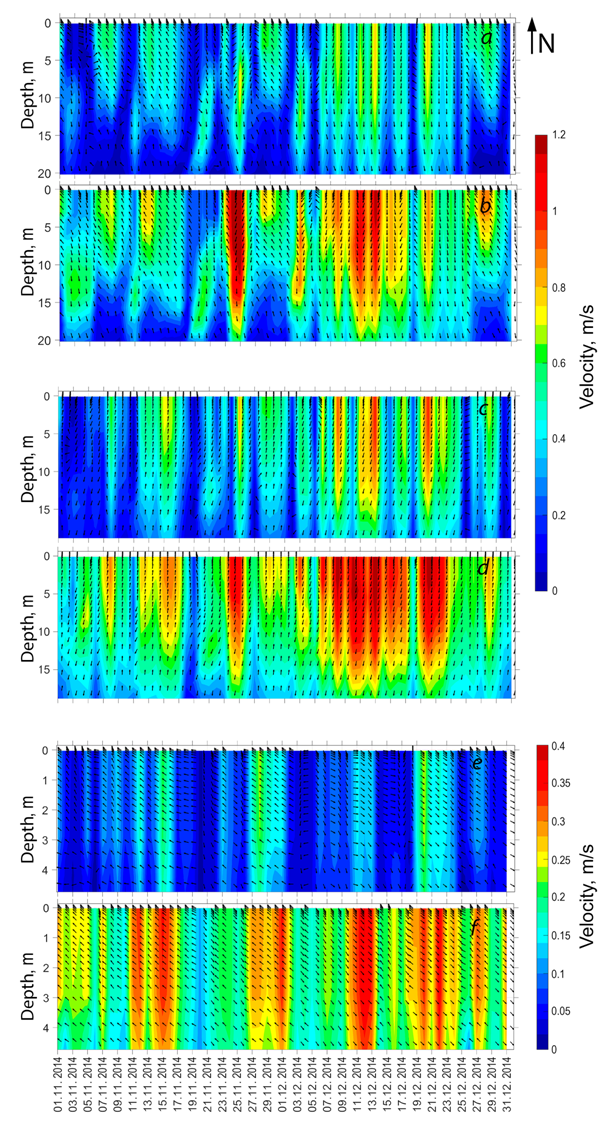
F i g. 5. Time variation of the daily average (а, c, e) and maximum (b, d, f) current velocity vectors at different horizons in the Sound (а, b), Great Belt (c, d) and Little Belt (e, f) straits calculated by the INMOM model for the period from 1 November to 31 December 2014 (see Fig. 1, b)
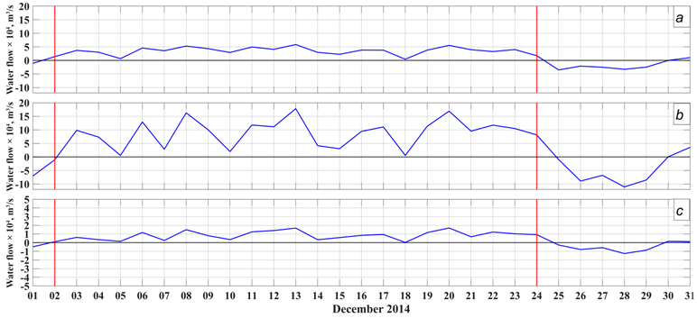

F i g. 6. Daily average flow rates of currents during the 2014 MBI in the Sound (a), Great Belt (b) and Little Belt (c) straits calculated based on the INMOM modeling results
T a b l e 3
Estimates of total volume of the salty North Sea waters (km3) flowing
to the Southwestern Baltic through the Danish straits during the 2014 MBI main period according to the INMOM modeling results and [5]
|
Straits |
INMOM |
[5] |
|
Sound |
68.9 |
64¸76 |
|
Great Belt |
170.9 |
205¸248* |
|
Little Belt |
1.6 |
No data |
|
Total |
241.4 |
281¸323 |
* The estimates included values of water exchange through the Little Belt Strait.
Table 3 shows the total volumes of the salty North Sea waters calculated based on the INMOM model simulation results that entered the Southwestern Baltic during the main MBI period (2–24 December 2014) through the Danish straits. For comparison, Table 3 shows the same estimates obtained by V. Mohrholz using other methods [5]. In contrast to our calculations of transport through the Danish straits carried out with formula (1), V. Mohrholz applied two indirect methods to estimate water exchange between the Kattegat and the Baltic Sea during the MBI of the year: based on changes in the Baltic water volume calculated using the water balance equation and based on sea level slopes between the Kattegat and the Southwestern Baltic [5]. He used both sea level measurements at tide gauge stations and the results of numerical hydrodynamic modeling as initial data for such estimates [5]. The transport estimates obtained using the INMOM model indicate that in December 2014, only 241.4 km3 of the Kattegat water passed through the Danish straits during the MBI. Its largest part passed through the Great Belt (170.9 km3) while only 68.9 km3 passed through the Sound. The Little Belt influence on the MBI water distribution turned out to be very insignificant (only 1.6 km3) (Table 3). These estimates are in good agreement with the conclusions in [35], according to which the volumes of water transport are distributed in the 7:3 ratio during large inflows between the Great Belt and the Sound. The results presented in Table 3 also show that our estimates of transport in the Sound are close to those obtained using other methods in [5] while for the Great Belt, our estimates of transport turned out to be somewhat smaller compared to the results in [5] (see Table 3).
Bottom salinity fields in the main MBI periods
Fig. 7 shows bottom salinity fields calculated using the INMOM model for four main periods of the 2014 MBI formation. During the outflow of the Baltic waters, the Sound is completely filled with the freshened Baltic waters with the 9–11‰ salinity (Fig. 7, a). Water masses with increased salinity of 17–20‰, which were there during previous weak inflows, are observed in the bottom layers of the Arkona and Bornholm basins (Fig. 7, a).
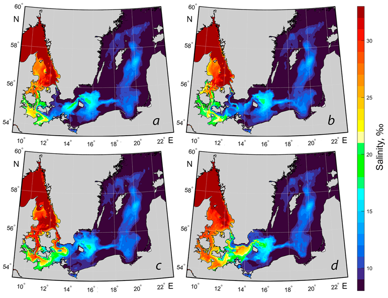
F i g. 7. Bottom salinity in four periods of the 2014 MBI formation: a – outflow period on 16.11.2014; b – precursory period on 01.12.2014; c – main inflow period on 12.12.2014; d – post inflow period on 29.12.2014
In the MBI preceding period, the outflow of the freshened Baltic waters through the Danish straits continues, resulting in a salinity decrease in Mecklenburg and Kiel bays and in the Little and Great Belts (Fig. 7, b). It is also evident that during this period, more saline bottom Arkona Basin waters move into the Sound, increasing the Arkona Basin water salinity (Fig. 7, b).
During the main inflow period, large volumes of the North Sea waters with the 30‰ salinity fill the Sound and Great Belt and spread further into the Southwestern Baltic (Fig. 7, c). From the Sound, they penetrate into the Arkona Basin and the northern part of the Bornholm, from the Great Belt – into Kiel and Mecklenburg bays as well as into the western part of the Belt Sea (Fig. 7, c). A very small amount of the salty North Sea waters enters through the Little Belt (Fig. 7, c).
In the period after the great inflow at the end of December 2014, almost the entire Arkona Basin, part of the Bornholm Basin, Kiel and Mecklenburg bays and the Belt Sea are filled with the transformed North Sea waters (Fig. 7, d). The salinity of the Sound and Great Belt waters decreases significantly.
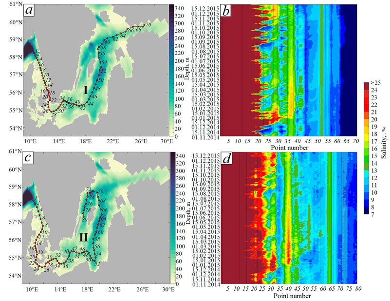
F i g. 8. Temporal variability of water salinity in the layer above the bottom on two sections: I (a, b) and II (c, d) based on the INMOM modeling data for the period from 1 November 2014 to 31 December 2015
Temporal changes in bottom salinity on sections across the open Baltic in 2014–2015
Fig. 8 demonstrates temporal variability in bottom salinity on two sections (Fig. 8, a, c) from 01.11.2014 to 31.12.2015. Spatio-temporal diagrams show that by mid-December 2014, after passing the Sound and the Great Belt, the salty MBI waters enter the Arkona Basin (Fig. 8, b, d), increasing the bottom salinity in it from 12 to 22–25‰ over the course of one and a half months until the end of January 2015. Then, the MBI waters spread into the Bornholm Basin where they enter in the first half of January 2015 with a salinity of 17–19‰ (Fig. 8, b, d). Comparison of Figs. 8, b and 8, d shows that the main route of the MBI water propagation passes north of Bornholm Island where a greater salinity increase to the south of it is observed.
The results given in Fig. 8, d show that in mid-February 2015, the transformed MBI waters enter the Gulf of Gdansk with the 12–13‰ salinity at the bottom. They spread then northward and enter the Gotland Deep in early April 2015 (Fig. 8, b, d). A further salinity increase in the bottom layer on section I is noted up to point 64, indicating that in 2015, the transformed MBI waters did not enter the Gulf of Finland. On section II, a salinity increase is observed up to point 71. These results demonstrate that the transformed MBI waters enter the western part of the Gotland Basin.
Trajectories of markers during the spread of MBI waters based on the Lagrangian modeling results
Fig. 9 shows the trajectories of markers placed in the southern Kattegat in November–December 2014 obtained with Lagrangian modeling. It can be seen that by the end of December 2014, most of the markers pass the Danish straits, the Arkona Basin and further enter the Bornholm Basin (Fig. 9, a) which is in good agreement with the results obtained by another method and presented in Fig. 8. A significant portion of the markers move from their placement site to the north of the Kattegat and penetrate the Skagerrak (Fig. 9, a). By the end of March 2015, the markers fill the Arkona and Bornholm basins almost completely and move in a wide flow to the east, to the Gulf of Gdansk. There, they split into two flows, the wider of which fills the Gulf of Gdansk actively, and the other, narrower, spreads north of the Gulf of Gdansk and moves to the Gotland Basin eastern part (Fig. 9, b). Another narrow flow spreads from the Bornholm Basin to the north-northeast (Fig. 9, b). By the end of July 2015, the markers moving in a wide flow penetrate in large numbers into the eastern part of the Gotland Basin and the Gotland Deep (Fig. 9, c). At the end of December 2015, they spread to the north of the open Baltic and, moving along a cyclonic trajectory, enter the Landsort Deep (Fig. 9, d).
Thus, two different methods of studying the December 2014 spread of transformed MBI waters indicate that its waters did not penetrate into the Gulf of Finland by the end of 2015 (see Figs. 8 and 9). These results are in good agreement with the estimates of the spread of the transformed Baltic Basin waters obtained in [36] using hydrochemical analysis of water samples on the oceanographic section between the Gotland Deep and the central part of the Gulf of Finland. Based on an analysis of the results of temperature, salinity and oxygen measurements at oceanographic stations, the authors of [36] note that nine months after the December 2014 MBI, deep stagnant waters from the northern part of the open Baltic, which were there before the MBI, were forced into the Gulf of Finland; the directly transformed waters of the 2014 MBI entered the Gulf of Finland only in 2016, 14–15 months after the MBI [36], but with very low oxygen content.
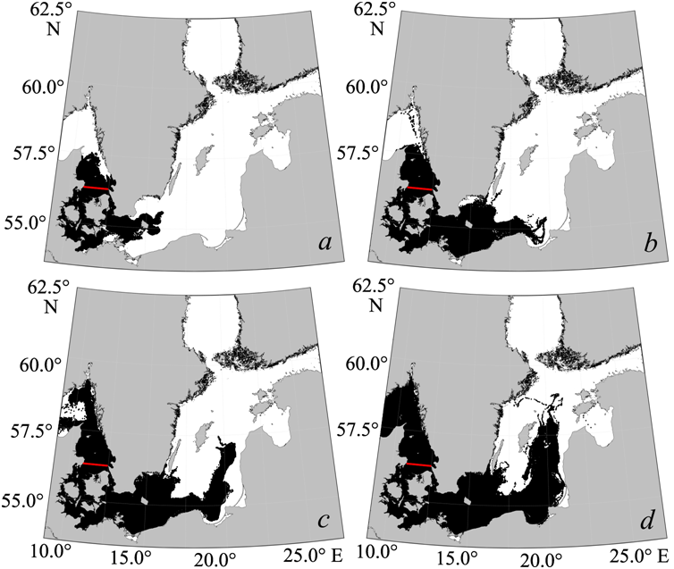
F i g. 9. Trajectories of the Lagrangian particles from the moment of launch up to 31 December 2014 (а); 31 March 2015 (b); 31 July 2015 (с); 31 December 2015 (d). Red line shows the place where the markers were launched
Conclusion
The performed study makes it possible to draw the following principal conclusions:
- According to the INMOM base model, a joint numerical baroclinic hydrodynamic model of the North and Baltic seas, having a spherical grid domain with detailing in the Danish straits, to study the MBI formation and propagation, was developed. Modeling of the variability of oceanographic conditions in the North and Baltic Sea system during the December 2014 MBI formation and propagation was carried out.
- To test the developed model performance, the model estimates were compared with the results of salinity and current measurements at different horizons of the Darss Sill and Arkona automatic stations as well as with the regional BSPAF reanalysis data implementing the NEMO 3.6 model. The comparison showed that the INMOM model reproduces salinity changes generally in the Southwestern Baltic better: in the Darss Sill station area, the values of the Pa accuracy criterion show that 43–57% of the salinity estimates calculated by INMOM fall within the range of measured values not exceeding 0.674s while, according to the BSPAF reanalysis, only 16–25% of the values fall within this range. For the Arkona station area, the estimates of accuracy criterion Pa based on the INMOM modeling results vary from 33 to 82% while according to the BSPAF reanalysis data, they do not exceed 7–49%. Comparison of statistical estimates of the calculated and measured characteristics of currents showed that the INMOM model reproduced the characteristics of average flows at different horizons during the 2014 MBI formation better while the BSPAF reanalysis data often described the characteristics of oscillatory movements in the deep and bottom layers more realistically.
- Modeling of oceanographic conditions during the 2014 MBI using the INMOM model shows that its main period started on 2–3 December 2014 and lasted until 24 December 2014. During it, unidirectional flows of the Kattegat waters into the Baltic Sea are observed in the Danish straits, decreasing with depth by 1.5–2 times in terms of velocity module, with maximum velocities reaching 1.2 m/s in the Sound and the Great Belt and only 0.4 m/s in the Little Belt. The movement nature of unidirectional flows of the Kattegat waters in the straits is not monotonous but fluctuating. Periods between current fluctuations vary from 2 to 4 days and current velocities change by 20–60 cm/s.
- The bottom salinity fields calculated using the INMOM model during the main periods of formation and spread of the major inflow of 2014 show that during the outflow of the Baltic waters, the Sound is completely filled with the freshened Baltic waters of the 9–11‰ salinity and in the bottom layers of the Arkona and Bornholm basins, water masses of increased salinity of 17–20‰, which spread here during previous weak inflows, are observed. In the precursory period, the outflow of the freshened Baltic waters through the Danish straits goes on, resulting in a salinity decrease in Mecklenburg and Kiel bays and in the Little Belt. The bottom waters from the Arkona Basin move to the Sound, resulting in the salinity decrease in the Arkona Basin. During the influx main period, large volumes of the North Sea waters with the 30‰ salinity fill the Sound and the Great Belt, penetrating into the Arkona Basin and the northern part of the Bornholm Basin as well as into Kiel and Mecklenburg bays and into the Belt Sea. A very small amount of the salty North Sea waters enters through the Little Belt.
- Water exchange estimates obtained using the INMOM model indicate that in December 2014, during the main MBI period, a total of 241.4 km3 of the Kattegat water passed through the Danish straits. The largest part of this was distributed through the Great Belt (170.9 km3), while only 68.9 km3 passed through the Sound. The Little Belt influence on water transport during the MBI was very insignificant – only 1.6 km3.
- A study of the propagation routes of the transformed North Sea waters across the Baltic after the MBI end on two sections with Lagrangian modeling shows that after passing the Danish straits, the MBI waters spread in a wide flow into the Southwestern Baltic, then penetrate into the Gulf of Gdansk and move further along a cyclonic trajectory through the deep-water areas of the eastern and northern parts of the Gotland Basin, without penetrating into the Gulf of Finland, and they reach the Landsort Deep in the western part of the Gotland Basin by the end of December 2015.
1. Dickson, R.R., 1973. The Prediction of Major Baltic Inflows. Deutsche Hydrographische Zeitschrift, 26, pp. 97-105. https://doi.org/10.1007/BF02232597
2. Terziev, F.S., Rozhkov, V.A. and Smirnova, A.I., eds., 1992. Hydrometeorology and Hydrochemistry of the Seas of the USSR. Volume 3. Baltic Sea. Issue 1. Hydrometeorological Conditions. Saint Petersburg: Gidrometeoizdat, 450 p. (in Russian).
3. Fischer, H. and Matthäus, W., 1996. The Importance of the Drogden Sill in the Sound for Major Baltic Inflows. Journal of Marine Systems, 9(3-4), pp. 137-157. https://doi.org/10.1016/S0924-7963(96)00046-2
4. Matthäus, W., 2006. The History of Investigation of Salt Water Inflows into the Baltic Sea – from the Early Beginning to Recent Results. In: Institut für Ostseeforschung, 2006. Meereswissenschaftliche Berichte = Marine Science Reports. Warnemünde: Institut für Ostseeforschung. No. 65, 73 p. URL: https://doi.io-warnemuende.de/10.12754/msr-2006-0065 [Accessed: 20.02.2025].
5. Mohrholz, V., Naumann, M., Nausch, G., Krüger, S. and Gräwe, U., 2015. Fresh Oxygen for the Baltic Sea – An Exceptional Saline Inflow after a Decade of Stagnation. Journal of Marine Systems, 148, pp. 152-166. https://doi.org/10.1016/j.jmarsys.2015.03.005
6. Tikhonova, N.A. and Sukhachev, V.N., 2017. Wave Interpretation of Major Baltic Inflows. Russian Meteorology and Hydrology, 42(4), pp. 258-266. https://doi.org/10.3103/S1068373917040069
7. Zakharchuk, E.A., Litina, E.N., Klevantsov, Yu.P., Sukhachev, V.N. and Tikhonova, N.A., 2017. Nonstationarity of the Hydrometeorological Processes in the Baltic Sea under Changing Climate. Proceedings of State Oceanographic Institute, (218), pp. 6-62 (in Russian).
8. Leppäranta, M. and Myrberg, K., 2009. Topography and Hydrography of the Baltic Sea. In: M. Leppäranta and K. Myrberg, 2009. Physical Oceanography of the Baltic Sea. Berlin; Heidelberg: Springer, pp. 41-88. https://doi.org/10.1007/978-3-540-79703-6
9. Zakharchuk, E.A., Kudryavtsev, A.S. and Sukhachev, V.N., 2014. On the Resonance-Wave Mechanism of Major Baltic Inflows. Russian Meteorology and Hydrology, 39(2), pp. 100-108. https://doi.org/10.3103/S1068373914020058
10. Wyrtki, K., 1953. Die Dynamik der Wasserbewegungen im Fehmarnbelt. Kieler Meeresforschungen, 9(2), pp. 155-170 (in German).
11. Madsen, K.S. and Højerslev, N.K., 2009. Long-Term Temperature and Salinity Records from the Baltic Sea Transition Zone. Boreal Environment Research, 14, pp. 125-131.
12. Gräwe, U., Friedland, R. and Burchard, H., 2013. The Future of the Western Baltic Sea: Two Possible Scenarios. Ocean Dynamics, 63(8), pp. 901-921. https://doi.org/10.1007/s10236-013-0634-0
13. Stigebrandt, A., 1983. A Model for the Exchange of Water and Salt between the Baltic and the Skagerrak. Journal of Physical Oceanography, 13(3), pp. 411-427. https://doi.org/10.1175/1520-0485(1983)013<0411:AMFTEO>2.0.CO;2
14. Meier, H.E.M., Kjellström, E. and Graham, L.P., 2006. Estimating Uncertainties of Projected Baltic Sea Salinity in the Late 21st Century. Geophysical Research Letters, 33(15), L15705. https://doi.org/10.1029/2006GL026488
15. Neumann, T., 2010. Climate-Change Effects on the Baltic Sea Ecosystem: A Model Study. Journal of Marine Systems, 81(3), pp. 213-224. https://doi.org/10.1016/j.jmarsys.2009.12.001
16. Hordoir, R., Dieterich, C., Basu, C., Dietze, H. and Meier, H.E.M., 2013. Freshwater Outflow of the Baltic Sea and Transport in the Norwegian Current: A Statistical Correlation Analysis Based on a Numerical Experiment. Continental Shelf Research, 64, pp. 1-9. https://doi.org/10.1016/j.csr.2013.05.006
17. Burchard, H., Lass, H.U., Mohrholz, V., Umlauf, L., Sellschopp, J., Fiekas, V., Bolding, K. and Arneborg, L., 2005. Dynamics of Medium-Intensity Dense Water Plumes in the Arkona Basin, Western Baltic Sea. Ocean Dynamics, 55(5), pp. 391-402. https://doi.org/10.1007/s10236-005-0025-2
18. Umlauf, L., Arneborg, L., Burchard, H., Fiekas, V., Lass, H.U., Mohrholz, V. and Prandke, H., 2007. Transverse Structure of Turbulence in a Rotating Gravity Current. Geophysical Research Letters, 34(8), L08601. https://doi.org/10.1029/2007GL029521
19. Lehmann, A. and Myrberg, K., 2008. Upwelling in the Baltic Sea – A Review. Journal of Marine Systems, 74(1), pp. S3-S12. https://doi.org/10.1016/j.jmarsys.2008.02.010
20. Fennel, W., Seifert, T. and Kayser, B., 1991. Rossby Radii and Phase Speeds in the Baltic Sea. Continental Shelf Research, 11(1), pp. 23-36. https://doi.org/10.1016/0278-4343(91)90032-2
21. Reißmann, J.H., 2006. On the Representation of Regional Characteristics by Hydrographic Measurements at Central Stations in Four Deep Basins of the Baltic Sea. Ocean Science, 2(1), pp. 71-86. https://doi.org/10.5194/os-2-71-2006
22. Osiński, R., Rak, D., Walczowski, W. and Piechura, J., 2010. Baroclinic Rossby Radius of Deformation in the Southern Baltic Sea. Oceanologia, 52(3), pp. 417-429. http://dx.doi.org/10.5697/oc.52-3.417
23. Kurkin, A., Kurkina, O., Rybin, A. and Talipova, T., 2020. Comparative Analysis of the First Baroclinic Rossby Radius in the Baltic, Black, Okhotsk, and Mediterranean Seas. Russian Journal of Earth Sciences, 20(4), ES4008. https://doi.org/10.2205/2020ES000737
24. Zhang, Y.J., Stanev, E.V. and Grashorn, S., 2016. Unstructured-Grid Model for the North Sea and Baltic Sea: Validation against Observations. Ocean Modelling, 97, pp. 91-108. https://doi.org/10.1016/j.ocemod.2015.11.009
25. Zalesny, V.B., Marchuk, G.I., Agoshkov, V.I., Bagno, A.V., Gusev, A.V., Diansky, N.A. Moshonkin, S.N., Tamsalu, R. and Volodin, E.M., 2010. Numerical Simulation of Large-Scale Ocean Circulation Based on the Multicomponent Splitting Method. Russian Journal of Numerical Analysis and Mathematical Modelling, 25(6), pp. 581-609. https://doi.org/10.1515/rjnamm.2010.036
26. Diansky, N.A., 2013. [Modeling the Ocean Circulation and Study of Its Response to Short- and Long-Period Atmospheric Influences]. Moscow: Fizmatlit, 272 p. (in Russian).
27. Brydon, D., Sun, S. and Bleck, R., 1999. A New Approximation of the Equation of State for Seawater, Suitable for Numerical Ocean Models. Journal of Geophysical Research: Oceans, 104(C1), pp. 1537-1540. https://doi.org/10.1029/1998JC900059
28. Pacanovsky, R.C. and Philander, G.H., 1981. Parametrization of Vertical Mixing in Numerical Models of Tropical Oceans. Journal of Physical Oceanography, 11(11), pp. 1443-1451. https://doi.org/10.1175/1520-0485(1981)011<1443:POVMIN>2.0.CO;2
29. Yakovlev, N.G., 2009. Reproduction of the Large-Scale State of Water and Sea Ice in the Arctic Ocean from 1948 to 2002: Part II. The State of Ice and Snow Cover. Izvestiya, Atmospheric and Oceanic Physics, 45(4), pp. 478-494. https://doi.org/10.1134/S0001433809040082
30. Hunke, E.C. and Dukowicz, J.K., 1997. An Elastic-Viscous-Plastic Model for Sea Ice Dynamics. Journal of Physical Oceanography, 27(9), pp. 1849-1867. https://doi.org/10.1175/1520-0485(1997)027<1849:AEVPMF>2.0.CO;2
31. Hordoir, R., Axell, L., Löptien, U., Dietze, H. and Kuznetsov, I., 2015. Influence of Sea Level Rise on the Dynamics of Salt Inflows in the Baltic Sea. Journal of Geophysical Research: Oceans, 120(10), pp. 6653-6668. https://doi.org/10.1002/2014JC010642
32. Pemberton, P., Löptien, U., Hordoir, R., Höglund, A., Schimanke, S., Axell, L. and Haapala, J., 2017. Sea-Ice Evaluation of NEMO-Nordic 1.0: A NEMO-LIM3.6-Based Ocean-Sea-Ice Model Setup for the North Sea and Baltic Sea. Geoscientific Model Development, 10(8), pp. 3105-3123. https://doi.org/10.5194/gmd-10-3105-2017
33. Nerger, L., Hiller, W. and Schröter, J., 2005. A Comparison of Error Subspace Kalman Filters. Tellus A: Dynamic Meteorology and Oceanography, 57(5), pp. 715-735. https://doi.org/10.3402/tellusa.v57i5.14732
34. Prants, S.V., Uleysky, M.Yu. and Budyansky, M.V., 2017. Lagrangian Oceanography: Large-Scale Transport and Mixing in the Ocean. Physics of Earth and Space Environments. Cham: Springer, 273 p. https://doi.org/10.1007/978-3-319-53022-2
35. Mattsson, J., 1996. Some Comments on the Barotropic Flow through the Danish Straits and the Division of the Flow between the Belt Sea and the Öresund. Tellus A: Dynamic Meteorology and Oceanography, 48(3), pp. 456-464. https://doi.org/10.3402/tellusa.v48i3.12071
36. Liblik, T., Naumann, M., Alenius, P., Hansson, M., Lips, U., Nausch, G., Tuomi, L., Wesslander, K., Laanemets J. [et al.], 2018. Propagation of Impact of the Recent Major Baltic Inflows from the Eastern Gotland Basin to the Gulf of Finland. Frontiers in Marine Science, 5, 222. https://doi.org/10.3389/fmars.2018.00222