


Immanuel Kant Baltic Federal University
Russian Federation
Russian Federation
Purpose. The paper is purposed at revealing the time periods since the mid-20th century when the annual average wave heights in the Baltic Sea tended to increase or decrease, assessing the statistical significance of potential time trends, as well as analyzing the statistical relationship between annual average wave heights in the Baltic Sea and the North Atlantic Oscillation. Methods and Results. The analysis is based on several points located in different parts of the Baltic Sea, in which the data on annual average wave heights cover the time intervals of several decades and are obtained by instrumental methods (one point), from field observations (two points) and modeling results (six points). The time series of annual average wave heights at these points are divided into the time segments of conditional monotony with predominant tendencies towards increase or decrease. The rates of change in wave heights at each segment and statistical significance of potential time trends are assessed using the non-parametric techniques. In the majority of cases, the trends within the segments under consideration are found to be statistically significant at the 90% level or more and the rates of change in the trend can range from 5 to 20 mm per year. The statistical relationship between annual average wave heights and the North Atlantic Oscillation is evaluated using the Pearson and Spearman correlation analysis. The correlation coefficients between the North Atlantic Oscillation indices and the annual average wave heights are statistically significant at the 90% level or more. Their numerical values within the interannual variability range constitute 0.3–0.6 and those between the five-year moving averages – 0.4–0.8. Conclusions. The increasing and decreasing phases in wave heights in the Baltic Sea alternate, at that each phase lasts 20 years. The time trends for each phase are statistically significant at least at some points in the sea. The correlation between the North Atlantic Oscillation index and the annual average wave heights is statistically significant but not high. Such correlation can account for 30–65% of the variations in wave characteristics
Baltic Sea, significant wave height, NAO index, time trend, statistical significance, correlation coefficient
Introduction
It can be considered that visual wind and wave situation observations in the Baltic Sea with its written recording have been carried out onboard vessels and in various parts of the coast since the early 19th century [1] when the well-known Beaufort scale for wind strength and wave height estimate appeared, later approved by the World Meteorological Organization . During visual observations, the attention is intuitively concentrated on relatively large waves with no regard for small ones, i.e. a certain general state of the sea is under estimation, not the height of individual waves [2, pp. 49–50]. Obviously, such estimates are quite subjective and far from being accurate. Instrumental measurements with precise recording of wave parameters began in the Baltic Sea only in the 1970s [3]. Modern wave recorders permit to determine both characteristics of individual waves passing through the point where the device is installed and statistical wave parameters, which can be correlated with the Beaufort scale.
One of the most important statistical characteristics of the waves is significant wave height (SWH), defined as the average height of one third of the highest waves recorded at a given point. This is the parameter that an experienced observer visually evaluates as the wave height. Later in the paper we will refer to significant wave heights and use the abbreviation SWH.
Many works have been devoted to the study of the Baltic Sea wave regime parameters [4]. However, most of them focus on the SWH spatial distribution. Temporal variability is analyzed in much fewer papers [1, 5–9].
The Baltic Sea wave regime parameters are related directly to global atmospheric circulation processes, in particular, to cyclonic activity. It is known [10, pp. 11–12] that the trajectories and intensity of atmospheric cyclones over the Atlantic and Europe are significantly affected by the North Atlantic Circulation (NAO). The typical state of the atmosphere over the North Atlantic is characterized by the Azores Maximum and the Iceland Minimum (in atmospheric pressure). If these extremes are clearly expressed (a large pressure difference is observed between them), a positive phase of the NAO takes place, otherwise – a negative one. For a quantitative estimate of the phenomenon, the NAO index is used. Its monthly average values from January 1950 to the present are published by the US Climate Prediction Center .
Works devoted to the analysis of the relationship between the North Atlantic Oscillation and wave heights in various water areas appeared in the 1990s. For example, in [11], the relationship between the SWH in the North Atlantic and the pressure gradient between the Azores Maximum and the Iceland Minimum in 1962–1988 is considered. The statistical relationship is noted both among the annual average and among the monthly average values of the quantities compared. Here, for the first time, an assumption that the North Atlantic Oscillation is primarily associated with the SWH interannual variability rather than long-term trends is made. This assumption for the North Atlantic and North Sea region is further developed in [12–14] and it is noted that the SWH annual average correlate better with the NAO indices averaged over the winter months (December – March) than the SWH monthly average and the monthly average NAO indices with each other.
Let us briefly touch on the works devoted to the study of the relationship between the North Atlantic Oscillation and wave heights in the Baltic Sea. In [7], based on the modeling data for 44 years (1958–2001), it is indicated that the relationship exists but no numerical values are given. In [5], a correlation (with a coefficient of 0.61) is noted between the annual average SWH off the Estonian coast for 1966–2006 and the NAO indices averaged over August–February period. At the same time, in [15], where the relationship between the annual average SWH off the coast of Poland for 1958–2002 and the annual average NAO indices as well as the monthly average SWH and the monthly average NAO indices is considered, the author concludes that although the relationship exists, it is quite weak.
In [16, 17], only storm events were considered. The relationship between annual average or monthly average SWH and NAO indices was not analyzed. The existence of a correlation at the 30–50% level between the number of storm events in the Baltic (with SWH > 2 m) and the NAO index was revealed.
Paper [18] analyzes the results of modeling the wave situation off the southern coast of Sweden for 62 years (1959–2021). It is noted that the interannual variability of the annual average energies and wave propagation directions is significantly correlated with the winter NAO indices (averaged for December – March). The statistical relationship is quantitatively measured by the Spearman correlation coefficient, which is 0.5–0.7 for different points in the coastal zone.
As can be seen from the brief review of published works, the existence of a correlation between the wave regime parameters in the Baltic and the NAO is beyond doubt but a number of questions remain open including the following: which of the NAO index averaging options shows the best correlation with the wave parameters and what is the degree of NAO influence on the wave parameters within the framework of interannual and multi-year variability.
In their previous works [8, 9], the authors considered the parameters of the Baltic Sea wave regime based on the results of numerical modeling for 1979–2018. Time trends in SWH changes in certain areas were identified and statistical significance of these trends was estimated. This paper is purposed at revealing the time periods since the mid-20th century when the annual average wave heights in the Baltic Sea tended to increase or decrease, assessing the statistical significance of potential time trends as well as analyzing the statistical relationship between annual average wave heights in the Baltic Sea and the North Atlantic Oscillation.
Materials and methods
Data used for the analysis. Let us consider the dynamics of wave heights in the Baltic Sea. Fig. 1 shows the location of the points and the time series of annual average SWH used for the analysis. The shades of gray reflect information about the spatial distribution of average SWH (for 1979–2018). The data on the time series of annual average SWH at points 1, 2 and 3 are taken from [1, 5, 6], at points 4–9 – results obtained by the authors. Below, the method for obtaining data for each of the points shown in Fig. 1 is considered in more detail.
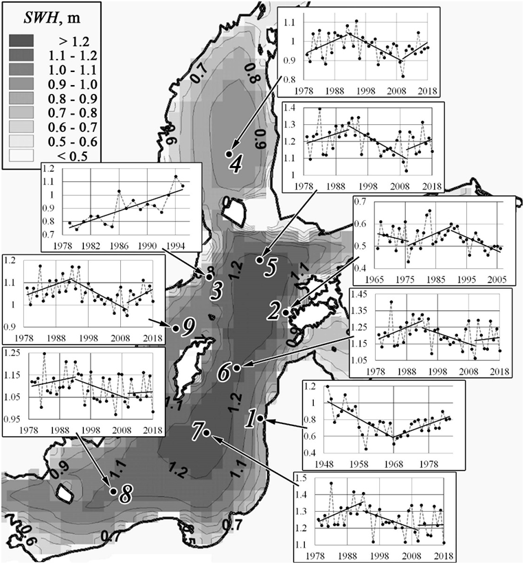
F i g. 1. Long-term dynamics of wave heights in the Baltic Sea. Color and isolines show the average SWH in the Baltic Sea based on numerical simulating data for 1979–2018 [8, 9]. White numerals highlight the points used in the study. Insets show the time series of annual average SWH for each point and the linear approximations for the areas that can be considered supposedly monotonic in visual analysis
Wave heights near the coast of Latvia in the Liepaja region (point 1 in Fig. 1) were estimated based on visual observations. Data on annual average SWH obtained using this method for 1949–1984 is presented in [6]. The time series in the inset for point 1 were constructed from these materials. The results given in [5] were used for the Estonian coast (point 2). The author of the study carried out calculations using a semi-empirical model based on the wave height dependence on the wave fetch. Data from the Vilsandi weather station located near the western end of Saaremaa Island were used to account for the wind effect. Annual average SWH calculations in this region (point 2) were carried out for the 1966–2006 period. Point 3 reflects the results of pioneering instrumental SWH measurements in the Baltic Sea at Almagrundet located several dozen kilometers from the Swedish coast. The results described in [1] cover the 1979–1995 period and form the basis for constructing a time series for point 3.
The time series for points 4–9 were obtained by the authors using the MIKE 21 SW spectral wave model for the 40-year period from 1979 to 2018. The unstructured computational grid covered the entire Baltic Sea. The side size of the triangular grid elements varied from 2–3 to 10–15 km. The model had no open boundaries. The time step during the calculations was adjusted by the model based on the stability condition but did not exceed 10 min. To take into account the wind effect, open ERA-Interim reanalysis data was used on a spatial grid of 1° in latitude and longitude with a time step of 6 hours. The model was calibrated and verified by comparing the calculation results with the data of wave buoys located in various parts of the Baltic Sea. Detailed information on the settings, calibration and verification of the model used for the calculations is given in [8, 9]. The choice of location of points 4–9 from the entire data set was due to the fact that they yielded the maximum significant wave heights for different Baltic Sea subregions according to model calculations for 1979–2018.
Analysis of temporal variability of annual average wave heights. The analysis of the dynamics of annual average SWH was carried out by studying their time series at the aforementioned points of the Baltic Sea. Each of the considered time series was subjected to processing including three stages.
At the first stage, time intervals were visually identified when the dependence of annual average SWH on time could be conditionally considered linear. The linear functions approximating them are shown as straight line segments in the insets. Then, for each of the identified intervals, the slope of the linear approximating function (Sen’s slope [19]) was determined using a non-parametric approach, and the statistical significance of the potential time trend was estimated using the Mann-Kendall Test [20, 21]. Statistical analysis was performed in Excel using the Real Statistics add-in for statistical significance level a = 0.1 (90% probability). At the last stage, statistical indicators for different spatial points were compared and conclusions about dynamics of annual average SWH in a particular time interval were made.
Estimate of relationship between annual average SWH and NAO index. The correlation of the time series of annual average SWH with the time series of the NAO index was analyzed for all the points shown in Fig. 1. The NAO index values used in this paper represent normalized pressure difference between the Gibraltar and Reykjavik (Iceland) weather stations. They are calculated using the method from [22] and their monthly average values are available online in the open database of the US Climate Prediction Center . These monthly average values were the initial data for the analysis of the relationship between NAO and wave height in the Baltic Sea.
In this study, both annual average NAO index values and its values averaged for various combinations of months from October to March were considered. Particular attention was paid to the cold months because winter processes of interaction between the ocean and the atmosphere have the greatest impact on the atmospheric circulation in the following months of the calendar year [23; 24; 10, p. 23]. For example, the most common averaging of the NAO index for winter months is abbreviated as JFM (January, February, March) which correlates well with various meteorological parameters [25, 26]. The works contain various options for averaging for October – March [27, 28].
The relationship was calculated using the Pearson and Spearman correlation coefficients (CC) In addition, the statistical significance of the calculated correlation coefficients was estimated for level a = 0.1. Statistical analysis was carried out in Excel using the Real Statistics add-in 5.
Results and discussion
Analysis of temporal variability of annual average SWH. Visual analysis (inserts in Fig. 1) shows that areas of decrease and increase in annual average SWH in the Baltic Sea alternate. From 1950 to the late 1960s – early 1970s, a decrease trend is observed. The rates of decrease range from 5 (point 2) to 23 (point 1) mm/year. This period is covered by very little data obtained mainly by visual observation. Therefore, the results are quite subjective and not very reliable.
Since the late 1960s – early 1970s, a tendency for annual average SWH to increase has been observed, which is confirmed by time series at all points. The rates of increase range from 6 (point 9) to 17 (point 3) mm/year. Significantly more data here were obtained by both visual and more objective methods – using instrumental measurements and mathematical modeling.
From the early 1990s until approximately 2010, a decrease trend in annual average SWH was observed again. This conclusion is based on both calculations of the authors (points 4–9) and the modeling results [5] for point 2. The rates of decrease vary from 4 mm/year for point 8 to 13 mm/year for point 5. Presumably, an increase phase began again in 2010 but since the period covered by the data is limited to 2018, it is incorrect to draw conclusions about the increase rates as the period is too short for the analysis.
T a b l e 1
Rate of annual average SWH change for the periods when the time trends can be considered statistically significant at level a = 0.1 (90% probability)
|
Point |
Period |
Trend is significant at a = 0.1 |
Trend value, mm/year |
|
1 |
1949–1968 |
yes |
−23.0 |
|
1968–1985 |
yes |
15.0 |
|
|
2 |
1966–1976 |
no |
– |
|
1976–1990 |
yes |
7.5 |
|
|
1990–2006 |
yes |
−6.0 |
|
|
3 |
1979–1995 |
yes |
17.0 |
|
4 |
1979–1992 |
no |
– |
|
1992–2010 |
yes |
−8.6 |
|
|
2010–2018 |
no |
– |
|
|
5 |
1979–1992 |
yes |
6.9 |
|
1992–2010 |
yes |
−13.0 |
|
|
2010–2018 |
no |
– |
|
|
6 |
1979–1993 |
yes |
8.8 |
|
1993–2010 |
yes |
−9.5 |
|
|
2010–2018 |
no |
– |
|
|
7 |
1979–1993 |
yes |
9.0 |
|
1993–2010 |
yes |
−8.3 |
|
|
2010–2018 |
no |
– |
|
|
8 |
1979–1993 |
no |
– |
|
1993–2010 |
yes |
−4.2 |
|
|
2010–2018 |
no |
– |
|
|
9 |
1979–1993 |
yes |
5.9 |
|
1993–2010 |
yes |
−7.6 |
|
|
2010–2018 |
no |
– |
To sum up, it can be assumed that the increase and decrease phases of annual average SWH in the Baltic have a duration of ~ 20 years: from 1950 to 1970 – decrease, from 1970 to 1990 – increase, from 1990 to 2010 – decrease. The rates of annual average SWH change vary spatially and can be ~ 5–20 mm/year.
In addition to calculating the rates of annual average SWH change, statistical significance of time trends was estimated for each of the time intervals under consideration. Calculations were carried out for level a = 0.1. The statistical significance of a potential time trend was estimated using the non-parametric Mann–Kendall method [20, 21] and the trend value was estimated using Sen’s slope formula [19]. Table 1 shows the calculation results.
The period up to the mid-1970s is presented in Table 1 only by points 1 (the Baltic coast near Liepaja, visual observations) and 2 (the western end of Saaremaa Island; a model based on the wave fetch). It is evident that for the period of SWH decrease from 1950 to the early to mid-1970s, the trend at point 1 is statistically significant, while at point 2 it is not. The absence of statistical significance at point 2 is explained, first of all, by the very short time period covered by the data (10 years of potential decrease in 1966–1976). For the increase period from the 1970s to the 1990s, data at all the points under consideration are available. The trend is statistically significant almost everywhere. The exceptions are points 4 (the Bothnian Sea) and 8 (the Bornholm Basin). Since the early 1990s, a decrease trend in SWH is observed again. It is statistically significant at all data points (all points except 1 and 3). For the period after 2010, a weak increase trend in SWH is observed and the trends are not statistically significant due to the short time interval covered by the data (8 years until 2018).
Estimate of relationship between annual average SWH and NAO index. To estimate the relationship, the correlation coefficients between the time series of annual average SWH and NAO indices averaged over different time intervals were calculated. The time series were not divided into segments of conditional monotonicity as in the trend analysis but the entire time series available at the point was taken as a whole. Table 2 presents the correlation analysis results. Statistical reliability of the given CCs is different: for minimal values of CCs, the p-value does not exceed 0.1 (i.e. probability of the statistical relationship existence is over 90%), for relatively high CCs (~ 0.5 and more), the p-value is 0.001 or less (99.9% probability).
For each of the time series, Table 2 shows at least one variant of averaging the NAO indices, in which the relationship with the annual average SWH is statistically significant at level a = 0.1. The highest CC values (0.3–0.6) are highlighted in bold. Most often (in all cases except point 2), the highest CC values correspond to the NAO index averaging period from January to March (JFM). This result coincides with the practice of using this averaging interval in scientific research. For example, on the US Climate Prediction Center website, this type of averaging, like no other, is the subject of a separate page
T a b l e 2
Pearson and Spearman correlation coefficients statistically significant at level a = 0.1 (90% probability)
|
Point |
Period |
CC |
Y |
JFM |
ONDJFM |
DJFM |
NDJFM |
|
1 |
1949–1976 |
Pearson (P.) |
– |
0.31 |
– |
– |
– |
|
Spearman (S.) |
– |
0.29 |
– |
– |
– |
||
|
2 |
1966–2006 |
P. |
0.29 |
- |
0.29 |
0.29 |
– |
|
S. |
0.33 |
- |
0.32 |
0.34 |
– |
||
|
3 |
1979–1995 |
P. |
– |
0.56 |
– |
– |
– |
|
S. |
– |
0.58 |
0.48 |
– |
0.47 |
||
|
4 |
1979–2018 |
P. |
0.41 |
0.60 |
0.31 |
– |
– |
|
S. |
0.33 |
0.53 |
– |
– |
– |
||
|
5 |
1979–2018 |
P. |
0.40 |
0.60 |
0.41 |
0.32 |
0.34 |
|
S. |
0.40 |
0.51 |
0.37 |
0.31 |
0.30 |
||
|
6 |
1979–2018 |
P. |
0.32 |
0.54 |
0.33 |
– |
– |
|
S. |
0.35 |
0.49 |
0.29 |
– |
– |
||
|
7 |
1979–2018 |
P. |
0.29 |
0.51 |
0.29 |
– |
– |
|
S. |
0.34 |
0.47 |
– |
– |
– |
||
|
8 |
1979–2018 |
P. |
– |
0.40 |
– |
– |
– |
|
S. |
– |
0.39 |
– |
– |
– |
||
|
9 |
1979–2018 |
P. |
0.34 |
0.53 |
0.37 |
0.28 |
0.28 |
|
S. |
0.35 |
0.47 |
0.37 |
0.30 |
0.27 |
N o t e. The Y column indicates the CCs between the annual average SWH and the annual average NAO indices. The remaining columns contain the CC values between the annual average SWH and the NAO indices averaged for different combinations of cold months of a year: O – October, N – November, D – December, J – January, F – February, M – March.
Thus, the calculations showed that the interannual variations of NAO and annual average SWH were in a statistically significant correlation. The second important thing was to find out which statistical relationship was more significant – for annual data or data with long time averaging. For this purpose, the CCs between the moving five-year averages of NAO indices and annual average SWH were additionally calculated. The calculations were carried out at all points for those cases of averaging for NAO indices that yielded the highest CC values when analyzing interannual variability. Table 3 demonstrates the results of the comparison of the correlation relationship.
T a b l e 3
Pearson and Spearman correlation coefficients between the NAO index annual values and the SWH annual average values as well as between their five-year moving averages
|
Point |
Period |
CC |
Annual values |
Five-year averages |
|
1 |
1949–1976 |
Pearson (P.) |
0.31 |
0.22 |
|
(JFM) |
Spearman (S.) |
0.29 |
0.38 |
|
|
2 |
1966–2006 |
P. |
0.29 |
0.36 |
|
(DJFM) |
S. |
0.34 |
0.41 |
|
|
3 |
1979–1995 |
P. |
0.56 |
0.71 |
|
(JFM) |
S. |
0.58 |
0.72 |
|
|
4 |
1979–2018 |
P. |
0.60 |
0.83 |
|
(JFM) |
S. |
0.53 |
0.82 |
|
|
5 |
1979–2018 |
P. |
0.60 |
0.76 |
|
(JFM) |
S. |
0.51 |
0.73 |
|
|
6 |
1979–2018 |
P. |
0.54 |
0.65 |
|
(JFM) |
S. |
0.49 |
0.58 |
|
|
7 |
1979–2018 |
P. |
0.51 |
0.58 |
|
(JFM) |
S. |
0.47 |
0.51 |
|
|
8 |
1979–2018 |
P. |
0.40 |
0.54 |
|
(JFM) |
S. |
0.39 |
0.50 |
|
|
9 |
1979–2018 |
P. |
0.53 |
0.73 |
|
(JFM) |
S. |
0.47 |
0.71 |
N o t e. The Period column specifies the option used for averaging the NAO index.
Table 3 shows that in all cases except for the Pearson CC for point 1, the CC for five-year averages is greater than for annual data, i.e. interannual SWH variations are statistically less significantly related to similar variations in NAO than longer-term ones. As for the spatial distribution, it is noteworthy that the CC for the offshore points is higher than the CC for the points near the coast. In addition, the SWH relationship with the North Atlantic Oscillation appears to increase from south to north: the highest CCs are calculated for points 3, 4, 5 and 9, with the strongest relationship for the northernmost point 4 in the Bothnian Sea.
Fig. 2 shows the SWH and NAO relationship by years as well as the effect of five-year averaging on the CC. Points 4 and 9 were chosen because the difference between the annual and five-year CCs is maximum for them – 0.2 or higher.
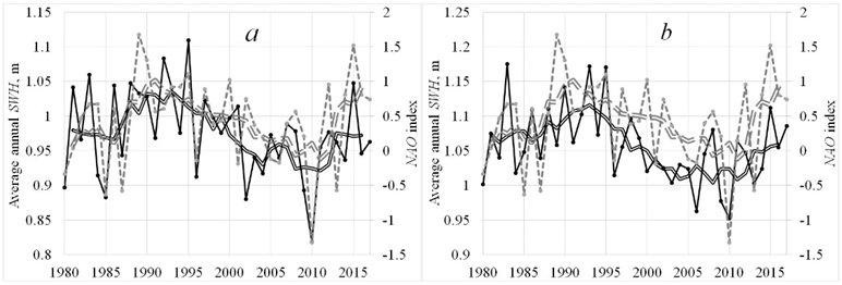
F i g. 2. Annual average SWH and NAO index averaged from January to March (JFM) for 1980–2017 at points 4 (a) and 9 (b). SWH: annual average values are indicated by a thin solid line, and five-year moving average – by a double solid line; NAO index (JFM): annual value is indicated by a dashed line, and five-year moving average – by a double dashed line
It can be seen from Fig. 2 that the fluctuations in the annual average SWH repeat the fluctuations in the annual NAO indices to a significant extent, which is confirmed by fairly high CCs for their interannual variations. Comparing the moving averages, it is easy to see that up to the early 1990s, an increase in both NAO indices and annual average SWH was observed. From the early 1990s until approximately 2010, a decrease in both annual average SWH and NAO indices took place. Finally, after 2010, both parameters have increase trends. Analyzing the results given in Fig. 2 and Table 3, it can be concluded that the NAO indices and the annual average SWH correlate both within the interannual variability and over longer time intervals.
Taking into account the determination coefficient (square of the correlation coefficient magnitude), showing in general terms what part of the analyzed variable (wave characteristic) variability can be explained using a regression model of its dependence on the NAO factor, it can be concluded that in the present case, the NAO influence can explain ~ 30–65% of the variability of wave characteristics both within the framework of interannual dynamics and over longer time periods.
The authors of this paper do not attempt to explain the mechanism of the NAO impact on wave height in the Baltic Sea physically. The paper estimates the relationship and, most importantly, evaluates its statistical significance, which allows, based on these evaluations, discussing possible mechanisms of the relationship (or declaring their insignificance).
Conclusion
1. The trends of increasing and decreasing annual average SWH in the Baltic Sea alternate. The duration of each of the conditional monotony phases is ~ 20 years. During the period from the mid-20th century to the 2020s, the trends changed three times.
2. The observed trends are statistically significant at level a = 0.1 (90% probability) at least at some points in the sea. The rates of annual average SWH change are small and can be 5–20 mm/year depending on the spatial position of the points.
3. The correlation between the NAO index and annual average wave heights is statistically significant at a level of at least 90% probability, but not high. This influence can explain ~ 30–65% of the change in wave characteristics both within the framework of interannual variability and over longer time periods.
4. The preferred averaging option for the NAO index, providing the highest correlation with annual average SWH, is in most cases the January to March (JFM) averaging.
1. Broman, B., Hammarklint, T., Rannat, K., Soomere, T. and Valdmann, A., 2006. Trends and Extremes of Wave Fields in the North-Eastern Part of the Baltic Proper. Oceanologia, 48(S), pp. 165-184.
2. Nesterov, E.S., ed., 2013. Regime, Diagnosis and Forecast of Wind Waves in the Oceans and Seas. Moscow: Hydrometeorological Research Center of Russian Federation, 292 p. (in Russian).
3. Tuomi, L., Kahma, K.K. and Pettersson, H., 2011. Wave Hindcast Statistics in the Seasonally Ice-Covered Baltic Sea. Boreal Environment Research, 16(6), pp. 451-472.
4. Soomere, T., 2023. Numerical Simulations of Wave Climate in the Baltic Sea: A Review. Oceanologia, 65(1), pp. 117-140. https://doi.org/10.1016/j.oceano.2022.01.004
5. Suursaar, Ü. and Kullas, T., 2009. Decadal Variations in Wave Heights near The Cape Kelba, Saaremaa Island, and Their Relationships with Changes in Wind Climate. Oceanologia, 51(1), pp. 39-61. https://doi.org/10.5697/oc.51-1.039
6. Soomere, T., 2013. Extending the Observed Baltic Sea Wave Climate back to the 1940s. Journal of Coastal Research, 65(sp. 2), pp. 1969-1974. https://doi.org/10.2112/SI65-333.1
7. Cieślikiewicz, W., Paplińska-Swerpel, B. and Soares, C.G., 2005. Multi-Decadal Wind Wave Modelling over the Baltic Sea. In: National Civil Engineering Laboratory, 2005. Coastal Engineering 2004: Proceedings of the 29th International Conference. Lisbon, Portugal: World Scientific Publishing Company, pp. 778-790. https://doi.org/10.1142/9789812701916_0062
8. Sokolov, A.N. and Chubarenko, B.V., 2020. Temporal Variability of the Wind Wave Parameters in the Baltic Sea in 1979–2018 Based on the Numerical Modeling Results. Physical Oceanography, 27(4), pp. 352-363. https://doi.org/10.22449/1573-160X-2020-4-352-363
9. Sokolov, A. and Chubarenko, B., 2024. Baltic Sea Wave Climate in 1979–2018: Numerical Modelling Results. Ocean Engineering, 297, 117088. https://doi.org/10.1016/j.oceaneng.2024.117088
10. Nesterov, E.S., 2013. [The North Atlantic Oscillation: Atmosphere and Ocean]. Moscow: Triada Ltd, 127 p. (in Russian).
11. Bacon, S. and Carter, D.J.T., 1993. A Connection between Mean Wave Height and Atmospheric Pressure Gradient in the North Atlantic. International Journal of Climatology, 13(4), pp. 423-436. https://doi.org/10.1002/joc.3370130406
12. Bauer, E., 2001. Interannual Changes of the Ocean Wave Variability in the North Atlantic and in the North Sea. Climate Research, 18(1-2), pp. 63-69. https://doi.org/10.3354/cr018063
13. Woolf, D.K., Challenor, P.G. and Cotton, P.D., 2002. Variability and Predictability of the North Atlantic Wave Climate. Journal of Geophysical Research: Oceans, 107(C10), 3145. https://doi.org/10.1029/2001JC001124
14. Dodet, G., Bertin, X. and Taborda, R., 2010. Wave Climate Variability in the North-East Atlantic Ocean over the Last Six Decades. Ocean Modelling, 31(3-4), pp. 120-131. https://doi.org/10.1016/j.ocemod.2009.10.010
15. Różyński, G., 2010. Long-Term Evolution of Baltic Sea Wave Climate near a Coastal Segment in Poland; Its Drivers and Impacts. Ocean Engineering, 37(2-3), pp. 186-199. https://doi.org/10.1016/j.oceaneng.2009.11.008
16. Surkova, G.V., Arkhipkin, V.S. and Kislov, A.V., 2015. Atmospheric Circulation and Storm Events in the Baltic Sea. Open Geosciences, 7(1), 20150030. https://doi.org/10.1515/geo-2015-0030
17. Myslenkov, S., Medvedeva, A., Arkhipkin, V., Markina, M., Surkova, G., Krylov, A., Dobrolyubov, S., Zilitinkevich, S. and Koltermann, P., 2018. Long-Term Statistics of Storms in the Baltic, Barents and White Seas and Their Future Climate Projections. Geography, Environment, Sustainability, 11(1), pp. 93-112. https://doi.org/10.24057/2071-9388-2018-11-1-93-112
18. Adell, A., Almström, B., Kroon, A., Larson, M., Uvo, C.B. and Hallin, C., 2023. Spatial and Temporal Wave Climate Variability along the South Coast of Sweden during 1959–2021. Regional Studies in Marine Science, 63, 103011. https://doi.org/10.1016/j.rsma.2023.103011
19. Sen, P.K., 1968. Estimates of the Regression Coefficient Based on Kendall’s Tau. Journal of the American Statistical Association, 63(324), pp. 1379-1389. https://doi.org/10.1080/01621459.1968.10480934
20. Mann, H.B., 1945. Nonparametric Tests against Trend. Econometrica, 13(3), pp. 245-259. https://doi.org/10.2307/1907187
21. Kendall, M.G., 1975. Rank Correlation Methods. London: Charles Griffin, 202 p.
22. Jones, P.D., Jonsson, T. and Wheeler, D., 1997. Extension to the North Atlantic Oscillation Using Early Instrumental Pressure Observations from Gibraltar and South-West Iceland. International Journal of Climatology, 17(13), pp. 1433-1450. https://doi.org/10.1002/(SICI)1097-0088(19971115)17:13%3C1433::AID-JOC203%3E3.0.CO;2-P
23. Hurrell, J.W., 1995. Decadal Trends in the North Atlantic Oscillation: Regional Temperatures and Precipitation. Science, 269(5224), pp. 676-679. https://doi.org/10.1126/science.269.5224.676
24. Rodwell, M.J., Rowell, D.P. and Folland, C.K., 1999. Oceanic Forcing of the Wintertime North Atlantic Oscillation and European Climate. Nature, 398, pp. 320-323. https://doi.org/10.1038/18648
25. Post, E. and Stenseth, N.C., 1999. Climatic Variability, Plant Phenology, and Northern Ungulates. Ecology, 80(4), pp. 1322-1339. https://doi.org/10.1890/0012-9658(1999)080[1322:CVPPAN]2.0.CO;2
26. D'Odorico, P., Yoo, J.C. and Jaeger, S., 2002. Changing Seasons: An Effect of the North Atlantic Oscillation. Journal of Climate, 15(4), pp. 435-445. https://doi.org/10.1175/1520-0442(2002)015<0435:CSAEOT>2.0.CO;2
27. Kolstad, E.W. and O’Reilly, C.H., 2024. Causal Oceanic Feedbacks onto the Winter NAO. Climate Dynamics, 62(5), pp. 4223-4236. https://doi.org/10.1007s00382-024-07128-y
28. Zhang, W. and Jiang, F., 2023. Subseasonal Variation in the Winter ENSO-NAO Relationship and the Modulation of Tropical North Atlantic SST Variability. Climate, 11(2), 47. https://doi.org/10.3390/cli11020047