


Russian Federation
Russian Federation
Purpose. The work is aimed at studying the changes in the thermal structure of the Black Sea upper layer during seasonal winter cooling in 2009−2010. Methods and Results. The NEMO-OASIS-WRF (NOW) coupled sea-atmosphere mesoscale model with the 2 km horizontal resolution is used. The changes in the sea upper layer during the 01.12.2009–28.02.2010 period are reproduced, and the temporal variability of water temperature at different depths is considered. For a characteristic point in the deep-sea part, it has been shown that the upper mixed layer thickness increased with time, whereas the cold intermediate layer upper boundary lowered as a result of the entrainment of colder water from below to the warmer upper mixed layer. It is also indicated that lowering of the cold intermediate layer upper boundary is accompanied by an increase of its temperature. In order to describe the cold intermediate layer evolution during winter cooling, two criteria are proposed: minimum water temperature in the 0−120 m layer, and difference between this value and the sea surface temperature. Vertical temperature profiles at different stages of winter cooling are obtained, and the main changes in thermal structure of the sea upper layer are considered. It is particularly shown that in course of winter cooling, the cold but less salty water at the northwestern shelf does not mix with the open sea waters due to a large horizontal density gradient. Conclusions. When describing the seasonal winter changes in the upper mixed layer, it is necessary to take into account not only heat transfer to the atmosphere through its upper boundary, but also the vertical turbulent exchange through its lower boundary. Heat accumulated over summer in the upper mixed layer is transferred not only to the atmosphere; its small part also goes to the lower levels, which leads to an increase of the cold intermediate layer temperature. The influence of boundary conditions, namely the inflow of waters with different features from the Marmara Sea, can lead to the formation of areas where the cold intermediate layer, though formally absent as a layer between two 8 °C isotherms, exists as an intermediate layer of colder (by 3−4 °C) water as compared to the upper mixed layer. During the 2009−2010 winter, vertical mixing including the transfer of warmer and less salty waters from the upper mixed layer to the lower ones was most intensive in the western part of the sea. This fact is assumed to be a result of the inhomogeneous sea cooling: heat flux directed from the sea surface to the atmosphere decreases from 200 W/m2 in the northwestern part of the sea up to 50 W/m2 in its southeastern part.
mesoscale coupled modeling, NOW sea-atmosphere model, cold intermediate layer, winter cooling, Black Sea
Introduction
A notable characteristic of the vertical structure of the upper layer of the northern seas is the presence of a low-temperature layer, which is the result of seasonal winter cooling from the sea surface. This layer is limited from below by a stable layer of increased salinity, known as the halocline, and is overlaid in summer by a warm upper mixed layer (UML) and a seasonal thermocline. The cold intermediate layer (CIL) is a distinctive feature of the northern seas, particularly in regions with relatively low winter temperatures. These include the North Atlantic, specifically the Baltic Sea, and the Black Sea.
The CIL development is based on the thermal structure of the upper sea layer, which is formed during the final stage of seasonal autumn-winter cooling. Following the termination of seasonal cooling, the cold layer can occupy the entire upper section of the sea up to the surface, thereby no longer serving as an intermediate layer. The subsequent development of this cold region, together with the onset of seasonal heating, and its subsequent formation as an intermediate layer located under the summer thermocline is influenced by various factors, including dissipation rates and advective processes within the layer itself. According to the processing data of buoy measurement results in the sea, the isolated CIL lifetime can reach two to three years [1].
The primary reason for the CIL renewal is linked to the uneven seasonal cooling of the upper Black Sea layer during the autumn-winter period. As is known, the most pronounced UMC cooling occurs in the central regions of the western and eastern cyclonic gyres within the deep-water part of the sea, while in the shallow areas, it is evident on the northwestern shelf (NWS) [2, 3]. These colder waters subsequently spread to the rest of the sea, descending along the main pycnocline to the periphery of the gyres and being transported by the alongshore Rim Current and the coastal mesoscale eddies associated with it [4–6]. In addition to long-term and gradual seasonal cooling, the Black Sea also experiences short periods of intense UML cooling during cold air intrusions (in the western part of the sea) [7, 8] and the Novorossiysk bora (in the eastern part) [9].
The cold intermediate layer in the Black Sea has exhibited considerable variation over time, manifesting interannual fluctuations. Studies of its interannual variability have been conducted repeatedly, using both observational data [10, 11] and numerical models [12]. These studies have revealed that in some years the CIL also experiences periods of absence. In the last decade, this tendency of significant weakening and even disappearance of the CIL has been discussed in the literature and is sometimes associated with global warming [13–15].
A typical example of the temporal variability of CIL is the period of 2009–2010. Below, the process of CIL destruction during the winter cooling of late 2009 – early 2010 will be examined. This process was reproduced in a coupled atmosphere-sea model with high spatial resolution. In our previous work [7], numerical experiments were carried out on a shorter time interval of 5 days to determine the sensitivity to individual physical mechanisms of deep penetrating cooling.
Numerical modeling in brief
The parameters selected for the NEMO-OASIS-WRF (NOW) coupled mesoscale model [16], consisting of the WRF atmospheric model and the NEMO marine model, are described in more detail in our previous works [7]. The spatial resolution of the coupled model was 2 km. The atmospheric model incorporated 37 vertical levels, while the marine model used 75 levels, with 38 of these levels located within the upper 100-meter layer. The Yonsei University scheme was employed to parameterize the planetary boundary layer in WRF and the Generic Length Scale scheme was used to parameterize vertical turbulent mixing in NEMO. Output interval of the modeling results was 1 hour. The initial conditions for the marine model, as well as the bottom topography, were taken from the Copernicus global reanalysis with a resolution of 1/12°, and the initial and boundary conditions for the atmospheric model were taken from the ERA5 reanalysis. The calculation was performed from December 1, 2009 to February 28, 2010. The atmospheric model employed a technique known as spectral “nudging”, which involves correction of atmospheric fields every 6 hours during the course of the modeling process, thereby aligning them with large-scale reanalysis fields.
Vertical structure of the upper sea layer
Figure 1 shows the time course of the sea surface temperature (SST) and the temperature at 60 and 80 m depths, along with the surface wind speed and the total (sensible + latent + shortwave + longwave) heat flux from the surface. It is evident (Fig. 1, c) that during the first two months of the seasonal winter cooling, the surface temperature demonstrated a consistent decline from 14 °C to a minimum of ~ 8 °C. The temperature graphs also show inertial oscillations with a period of ~ 17 h.
A notable feature that deviates from the prevailing trend of upper layer cooling is evident in two episodes of a sharp increase in the rate of decrease in SST: December 12–16, 2009, and particularly January 22–27, 2010 (highlighted in Fig. 1 with black circles). These episodes are accompanied by a sharp increase in surface wind speed and an increase in the heat flux from the sea surface to the atmosphere (Fig. 1, a, b). The latter episode, characterized as a case of cold air intrusion into the atmosphere of the Black Sea region, has been previously studied [7].
Figure 1, c also shows that in December and January the SST variations (sst graph) do not affect the CIL temperature (t60 and t80 graphs). However, beginning in February, the SST has dropped below 8 °C, and the temperature fluctuations at the three levels have occurred in approximately the same phase. This indicates that the vertical mixing in February covers the entire upper layer, extending down to the 80 m depth.
Figure 2 illustrates the changes in the vertical structure of the temperature field throughout the considered period of winter cooling. The upper mixed layer is clearly visible, exhibiting a decline in temperature to 8 °C with the depth increase from the initial value of 35 m to > 50 m. A notable characteristic of the CIL transformation is its reduction in thickness, leading to its dissolution as an intermediate cold layer. The observed decrease in CIL thickness is due to the lowering of the upper boundary of this layer.
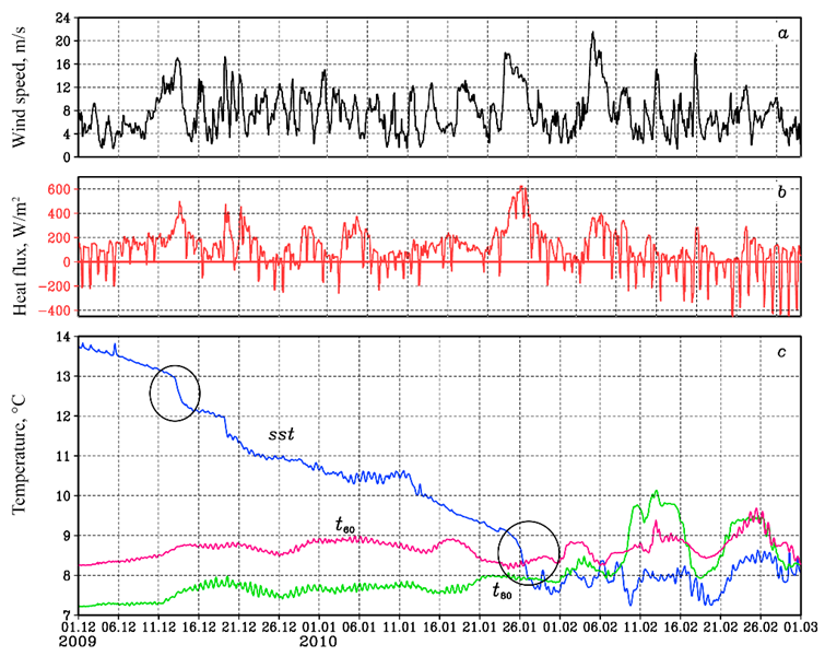
F i g. 1. Temporal changes of wind speed at the 10 m height (a), total heat flux (b) and water temperature at the surface and at depths 60 and 80 m (c) at point 32°E, 43.5°N for the period 01.12.2009–28.02.2010 (two cases of sharp drops in sea surface temperature are highlighted by black circles)
The nature of the change in the upper layer parameters during seasonal cooling is demonstrated more clearly by the vertical profiles of temperature, salinity gradient dS/dz and buoyancy frequency N, as shown in Fig. 3 for the same point as in Fig. 2. The profiles are shown for three successive moments of time: December 3, 2009 (the beginning of the calculation period), January 20, 2010 (the middle of the period, immediately before the beginning of the last episode of cold invasion) and February 28, 2010 (the end of the calculation period). The aforementioned feature of CIL transformation at the final stage of its disappearance is clearly visible. The physical mechanism of this phenomenon, i.e., the lowering of its upper boundary, is the entrainment of colder water into the warmer UML. It should be noted that the mechanism of entrainment at the lower UML boundary at the initial stage of autumn deepening is well-known and has been the subject of many studies [17].
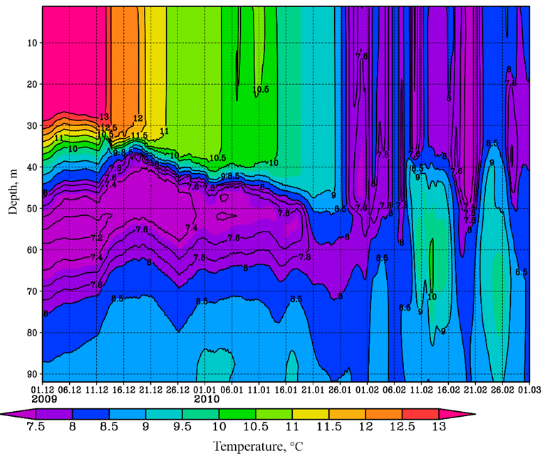
F i g. 2. Change in vertical temperature profiles at point 32°E, 43.5°N for the period 01.12.2009–28.02.2010. The temperature field is smoothed over time using a sliding average of 17 points
Lowering of the upper CIL boundary in December and January is accompanied by an increase in the halocline (Fig. 3, b). In contrast to temperature, water salinity is predominantly influenced by advection and vertical mixing, with the effect of evaporation from the sea surface being negligible. Over the duration of three months, the total change in salinity at the sea surface in the specified area was < 2% (for comparison, the SST change was ≈ 40%). It is evident that, even after the first month of calculation, the water temperature at the point of interest changes slightly with depth (Fig. 3, a), and stable stratification in the 40–60 m layer is ensured exclusively by the vertical salinity gradient. According to Fig. 3, b, c, the dS/dz and N graphs for January and February are very similar.
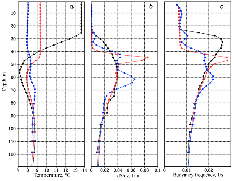
F i g. 3. Profiles of temperature (a), vertical salinity gradient (b) and buoyancy frequency (c) at point 32°E, 43.5°N in December (black curve) 2009, January (red curve) and February (blue curve) 2010
The buoyancy frequency graphs describe the CIL disappearance well. As the temperature equalizes with depth, it is evident that the buoyancy frequency decreases (Fig. 3, c). The N maximum falls on the lower boundary of the UML, and as this layer deepens, it also shifts downwards.
Figures 2, 3 show that the lowering of the upper CIL boundary is accompanied by an increase in its temperature. Over the course of two months, the minimum temperature in the CIL at the point under consideration increased from 7 to 8 °C. Consequently, during the seasonal UML cooling phase, a portion of the heat accumulated during summer does not fully escape into the atmosphere. Instead, some of this heat is transferred to the underlying levels, resulting in a reduction in the cold reserve of the CIL and its subsequent disappearance as an intermediate layer in depth.
Spatial structure of CIL
The spatial distribution of the CIL in the Black Sea is not as easily delineated as the individual parameters of the marine environment, such as temperature or salinity. This is due to the uncertainty and variability of the determining parameters. Traditionally, CIL in the Black Sea has been defined as a layer within the boundaries of the 8 °C isotherms. However, recently the criteria of 8.35 and 8.7 °C have also been used [18]. The average depth of the CIL in the Black Sea is 60 m, but in coastal regions it can reach depths of 100–120 m. To illustrate the changes in the spatial distribution of the CIL in the Black Sea, the water temperature fields at different depths are examined directly, rather than relying on formal criteria.
Figure 4, a, c, e, shows the spatial distribution of the minimum water temperature (tmin) in the upper 120 m layer, which is essentially the CIL core temperature, on 1 December 2009, 10 January and 26 February 2010. The arrows indicate the currents at the 20 m depth. Figure 4, b, d, f, shows the difference (∆t) between tmin and sea surface temperature for the aforementioned time moments. The ∆t can be considered as the temperature difference between the UML and the CIL core. This value may be crucial when contemplating the role of the CIL in regulating heat and mass exchange between the UML and the halocline.
Figure 4, a, b, shows that at the beginning of intense winter cooling in the shallow part of the sea north of 44.5°N, as well as along the western and southwestern coast, the water temperature in the entire layer down to the bottom was above 11−12 °C. In the areas where depth < 30 m, the water is well mixed vertically, and the temperature difference |∆t| < 0.1 °C. In the deep-water part, the CIL is well expressed: the temperature of its core is 7−8 °C, and the ∆t varies from −8 to −4 °C. An exception to this phenomenon is observed in the southwestern part of the sea, where tmin values are relatively large: temperature from the surface to a depth of 120 m is above 9−10 °C, i.e., formally, the CIL is absent. The underlying cause of this anomaly is attributed to the inflow of warmer and saltier waters from the Sea of Marmara, resulting in the presence of deep positive anomalies in the temperature and salinity fields. It is noteworthy that these anomalies are present in the initial conditions of the NEMO marine model, as represented by the Copernicus data. Based on Fig. 4, a, b, the absence of a formal CIL as a layer between the 8 °C isotherms does not necessarily imply the absence of a temperature difference with depth. In the regions of increased tmin values, the temperature difference between the intermediate layer core and the UML can reach 4 °C.
The modeled field of near-surface currents contains known features of the Black Sea circulation. In particular, in Fig. 4, a, coastal anticyclonic eddies in the Rim Current area, such as the Sevastopol, Kaliakra and Bosphorus gyres with centers at (32.5°E, 44.5°N), (29.2°E, 43.7°N) and (28.5°E, 42.5°N), as well as a cyclonic gyre specific for winter in the southeastern corner of the sea (41°E, 42°N), are distinguished.
Figure 4, c, d shows the same fields as Fig. 4, a, b, but one and a half months after the calculation period began. As can be seen, in the northern part of the sea, there is still a clear boundary between the warmer and less salty waters of the NWS and the coastal area and the denser waters of the open sea. The water temperature in the shallow part is still relatively high, > 9 °C, and only north of 44.5° N, where depth < 30 m, cold waters with a temperature of 6−7 °C are observed. In the deep part of the sea, the |∆t| value is found to be less than at the beginning of the calculation, with a range of 2 to 4 °C.
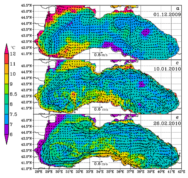
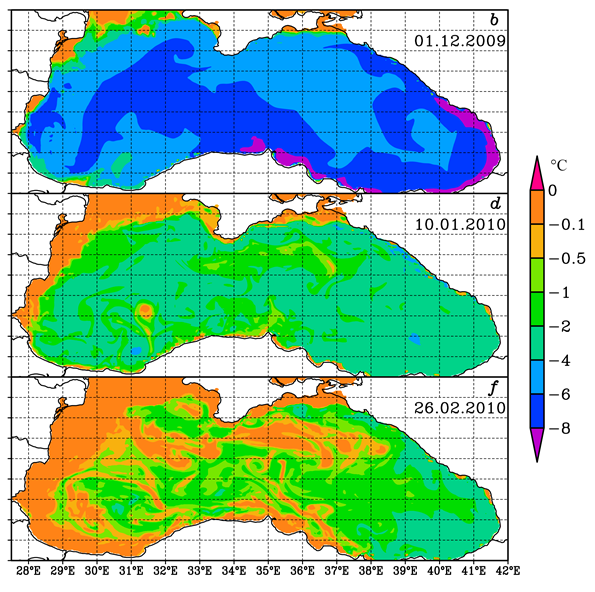
F i g. 4. Minimum water temperature, tmin, in the 0–120 m layer (left) and difference tmin − SST (right). Vectors show current velocity at the 20 m depth
Figure 4, c, e shows the impact of the currents on the spatial distribution of the water temperature. The influence of the Black Sea Rim Current caused an anomaly of warm salt water from the southwestern part to shift along the coast to the central and southeastern parts of the sea. This anomaly was slightly captured by the western cyclonic gyre (WCG), which led to the emergence of small positive anomalies of tmin in the southwestern part of the sea, even after the main anomaly shifted to the east.
Figure 4, b, d, f illustrates the dissipation of the CIL in the deep-water part of the sea, attributable to winter cooling and vertical mixing. According to Fig. 4, f, two months after the start of the calculations along the northern branch of the Rim Current, in the Kerch cyclonic gyre (36°E, 44.5°N), as well as on the WCG periphery, |Δt| did not exceed 0.1 °C. In this region, the temperature was equalized in depth within the upper 120-meter layer, leading to the dissipation of the CIL. Following two months of winter cooling, the CIL was best preserved in the southeastern part of the sea, where the temperature difference ranged from −4 to −2 °C. In contrast, in the western part, the absolute value of Δt did not exceed 2 °C.
The subsequent analysis will address the changes in the vertical structure of the temperature field throughout the sea during seasonal cooling. Figures 5 and 6 show the temperature fields for three distinct time moments on vertical sections drawn along 43.5°N and 31.5°E. As illustrated in Fig. 5, in the eastern part of the sea, with the exception of the area near the Caucasian coast, the upper boundary of the CIL is located at a slightly higher level than in the western part. The difference in occurrence depth reaches 10 m. Figure 5, a, b demonstrates the lowering of the upper boundary of the CIL during seasonal cooling, attributable to the increase in UML thickness. In the region west of 31°E, the UML thickness increased by 10 m over the span of nearly a month and a half (Fig. 5, b). In contrast, in the eastern part, the lowering of the upper boundary of the CIL is negligible due to the rise of 8–9 m in the layer core, caused by the intensification of the eastern cyclonic circulation during winter. In the western part, the rise in the cold-sea layer core was less pronounced, with an increase of 3–4 m.
Two months after the calculation start, the CIL remained predominantly in the eastern part of the sea, with a depth of 40–50 m within the 35–38°E region and 80–90 m near the Caucasian coast (Fig. 5, c). It is noteworthy that by the end of the calculation, a warm intermediate layer had already formed in certain areas at depths of 60 m. This layer consists of water with a higher (> 0.5–1 °C) temperature compared to the SST, explained by the strengthening of the main halocline during seasonal cooling and the subsequent vertical mixing.
As illustrated in Figs. 4, 5, the mixing of warmer and fresher waters from the UML to the underlying levels appears to have been most intense in the western part of the sea. This may be due to the uneven cooling of the sea during the period under consideration. It is indicated that the heat flux directed from the sea surface to the atmosphere decreases from 200 W/m2 in the northwestern part of the sea to 50 W/m2 in the southeastern one (not shown). This, in turn, is due to the non-uniform distribution of surface wind speed and air temperature. In the northwestern part, the mean values of wind speed and air temperature, averaged over a period of time, were ~ 10 m/s and 0 °C, in the southeastern part these values were ~ 5 m/s and 10 °C.
The heat flux from the surface (Q) is one of the two primary factors changing the SST in combination with vertical mixing [7]. The change in the UML temperature can be calculated by adding up the quantities , where Cp and ρ represent the heat capacity and seawater density, respectively; hi is the thickness of the mixed layer at the i-moment in time (defined in the model as the level depth below which the turbulent exchange coefficients are negligible); Qi denotes the heat flux at the i-moment in time; 3600 s is the time step with which the modeling results were output. For the section in Fig. 5, c, the decline in temperature over a period of two months is ~ 4.5−5 °C in the western and 3.5−4 °C in the eastern deep-water part of the sea.
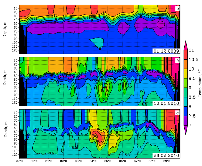
F i g. 5. Water temperature on a vertical section along 43.5°N for the same periods as in Fig. 4. Land is shaded in black
The vertical structure of the temperature and density fields in the NWS region was analyzed over time on a meridional section drawn along 31.5°E (Fig. 6). At the beginning of the calculation, to the south of 42.5°N, the area of waters with relatively high temperatures, as shown in Fig. 4, a, was clearly delineated. The average depth of the CIL on the section is 60 m, and its core temperature varies from 7–7.5 °C in the northern part of the section to 9–10 °C in the southern. The temperature difference between the CIL and the UML is significant even in the southern part, reaching 3–4 °C (Fig. 6, a).
As the seasonal cooling develops in the coastal region, a deflection of the primary pycnocline emerges and intensifies within the area of the continental slope (Fig. 6, c). Subsequently, following the winter cooling, the coastal region experiences an accumulation of relatively warm water, with the temperature 1°C higher than the surrounding environment (44.5–44.7°N). The eastern current velocity in this area also reaches high values, up to 0.6 m/s (not shown). Apparently, the elevated temperature values in the area of the continental slope are maintained by the Rim Current, which transports warm water (Fig. 4, e). At the same time, the cold water of the NWS does not mix with the waters of the open sea due to the presence of a large horizontal density gradient (Fig. 6, c).
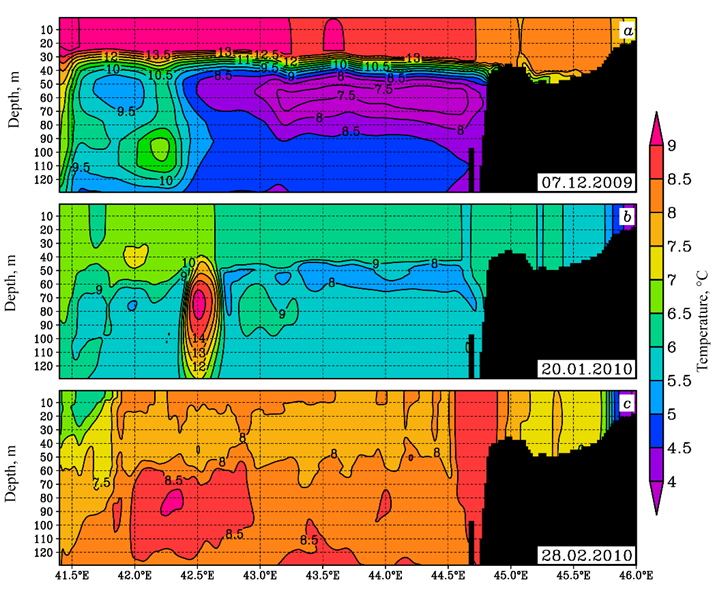
F i g. 6. Water temperature on a vertical section along 31.5°E. Land is shaded in black
It should be noted that the considered example and the CIL development features refer to a period in which the winter cooling was sufficiently intense to allow deep penetrating cooling to occur within the CIL area. In the case of a warmer winter season, the subsequent CIL development in the following year occurs in the context of a cold layer preserved underneath it.
Conclusion
The present paper explores the evolution of the CIL during seasonal cooling, using the winter of 2009–2010 as a case study. It has been demonstrated that when describing the seasonal winter changes in the UML, it is necessary to take into account not only the heat transfer to the atmosphere through the upper boundary, but also the vertical turbulent exchange through the lower boundary. This process leads to a gradual increase in the CIL temperature and a decrease in thickness due to the upper boundary lowering.
During the winter cooling season, the penetration of colder and saltier waters into the UML results in the strengthening of the halocline at depths of 40–60 m. This phenomenon ensures the preservation of high values of buoyancy frequency in the upper layer, despite the almost complete disappearance of the vertical temperature gradient.
It has been demonstrated that the influence of boundary conditions, manifesting as an inflow of waters with distinct properties from the Sea of Marmara, can significantly change the spatial distribution of the CIL. In the regions characterized by elevated temperatures, the CIL, despite its formal absence as a layer between two 8 °C isotherms, manifests as an intermediate layer of colder water (> 3−4 °C) in comparison to the UML. During this period, with minor exceptions, the cold intermediate layer occupies the greater portion of the sea.
A comparison of the western and eastern parts of the sea reveals a difference in the intensity of mixing. Following a two-month period of winter cooling, the CIL remained predominantly in the southeastern part. This can be due to the uneven cooling of the sea during the specified period. The heat flux directed from the sea surface to the atmosphere was ~ 200 W/m2 in the northwestern part of the sea and ~ 50 W/m2 in the southeastern part.
The modeled zonal temperature sections demonstrate that, in the western part of the sea, seasonal cooling resulted in an increase in the UML thickness. In the eastern part, the UML thickness increase was accompanied by an intensive rise in the main core of the CIL due to the activation of the winter circulation in the Black Sea.
The meridional sections of temperature, density, and current velocity demonstrate that, in the case under consideration, the vertical distribution of temperature in the northwestern part of the sea, in the area of the continental slope, was determined mainly by the warm Black Sea Rim Current
1. Akpinar, A., Fach, B.A. and Oguz, T., 2017. Observing the Subsurface Thermal Signature of the Black Sea Cold Intermediate Layer with Argo Profiling Floats. Deep Sea Research Part I: Oceanographic Research Papers, 124, pp. 140-152. https://doi.org/https://doi.org/10.1016/j.dsr.2017.04.002
2. Ivanov, L.I., Beşiktepe, Ș. and Özsoy, E., 1997. The Black Sea Cold Intermediate Layer. In: E. Özsoy and A. Mikaelyan, eds., 1997. Sensitivity to Change: Black Sea, Baltic Sea and North Sea. Dordrecht: Springer, pp. 253-264. https://doi.org/10.1007/978-94-011-5758-2_20
3. Ovchinnikov, I.M. and Popov, Yu.I., 1987. Evolution of the Cold Intermediate Layer in the Black Sea. Oceanology, 27(5), pp. 739-746.
4. Stanev, E.V., Bownam, M.J., Peneva, E. and Staneva, J.V., 2003. Control of Black Sea Intermediate Water Mass Formation by Dynamics and Topography: Comparison of Numerical Simulations, Surveys and Satellite Data. Journal of Marine Research, 61(1), pp. 59-99. https://doi.org/10.1357/002224003321586417
5. Staneva, J.V. and Stanev, E.V., 1997. Cold Intermediate Water Formation in the Black Sea. Analysis on Numerical Model Simulations. In: E. Özsoy and A. Mikaelyan, eds., 1997. Sensitivity to Change: Black Sea, Baltic Sea and North Sea. Dordrecht: Springer, pp. 375-393. https://doi.org/10.1007/978-94-011-5758-2_29
6. Korotayev, G.K., Knysh, V.V. and Kubryakov, A.I., 2014. Study of Formation Process of Cold Intermediate Layer Based on Reanalysis of Black Sea Hydrophysical Fields for 1971–1993. Izvestia, Atmospheric and Oceanic Physics, 50(1), pp. 35-48. https://doi.org/10.1134/S0001433813060108
7. Efimov, V.V. and Yarovaya, D.A., 2024. Numerical Modeling of the Black Sea Response to the Intrusion of Abnormally Cold Air in January 23–25, 2010. Physical Oceanography, 31(1), pp. 120-134.
8. Efimov, V.V. and Yarovaya, D.A., 2014. Numerical Simulation of Air Convection in the Atmosphere during the Invasion of Cold Air over the Black Sea. Izvestia, Atmospheric and Oceanic Physics, 50(6), pp. 610-620. https://doi.org/10.1134/S0001433814060073
9. Efimov, V.V., Komarovskaya, O.I. and Bayankina, T.M., 2019. Temporal Characteristics and Synoptic Conditions of Extreme Bora Formation in Novorossiysk. Physical Oceanography, 26(5), pp. 361-373. https://doi.org/10.22449/1573-160X-2019-5-361-373
10. Belokopytov, V.N., 2011. Interannual Variations of the Renewal of Waters of the Cold Intermediate Layer in the Black Sea for the Last Decades. Physical Oceanography, 20(5), pp. 347-355. https://doi.org/10.1007/s11110-011-9090-x
11. Dorofeev, V.L. and Sukhikh, L.I., 2017. Study of Long-Term Variability of Black Sea Dynamics on the Basis of Circulation Model Assimilation of Remote Measurements. Izvestia, Atmospheric and Oceanic Physics, 53(2), pp. 224-232. https://doi.org/10.1134/S0001433817020025
12. Miladinova, S., Stips, A., Garcia-Gorriz, E. and Macias Moy, D., 2017. Black Sea Thermohaline Properties: Long-Term Trends and Variations. Journal of Geophysical Research: Oceans, 122(7), pp. 5624-5644. https://doi.org/10.1002/2016JC012644
13. Demyshev, S.G., Korotaev, G.K. and Knysh, V.V., 2002. Evolution of the Cold Intermediate Layer in the Black Sea According to the Results of Assimilation of Climatic Data in the Model. Physical Oceanography, 12(4), pp. 173-190. https://doi.org/10.1023/A:1020156026089
14. Miladinova, S., Stips, A., Garcia-Gorriz, E. and Macias Moy, D., 2018. Formation and Changes of the Black Sea Cold Intermediate Layer. Progress in Oceanography, 167, pp. 11-23. https://doi.org/10.1016/j.pocean.2018.07.002
15. Stanev, E.V., Peneva, E. and Chtirkova, B., 2019. Climate Change and Regional Ocean Water Mass Disappearance: Case of the Black Sea. Journal of Geophysical Research: Oceans, 124(7), pp. 4803-4819. https://doi.org/10.1029/2019JC015076
16. Samson, G., Masson, S., Lengaigne, M., Keerthi, M. G., Vialard, J., Pous, S., Madec, G., Jourdain, N. C., Jullien, S., Menkes, C. and Marchesiello, P., 2014. The NOW Regional Coupled Model: Application to the Tropical Indian Ocean Climate and Tropical Cyclone Activity. Journal of Advances in Modeling Earth Systems, 6(3), pp. 700-722. https://doi.org/10.1002/2014MS000324
17. Kraus, E.B. and Turner, J.S., 1967. A One-Dimensional Model of the Seasonal Thermocline II. The General Theory and Its Consequences. Tellus, 19(1), pp. 98-106. https://doi.org/10.1111/j.2153-3490.1967.tb01462.x
18. Morozov, A.N. and Mankovskaya, E.V., 2020. Cold Intermediate Layer of the Black Sea according to the Data of the Expedition Field Research in 2016–2019. Ecological Safety of Coastal and Shelf Zones of Sea, (2), pp. 5-16. https://doi.org/10.22449/2413-5577-2020-2-5-16 (in Russian).