


Russian Federation
Russian Federation
Purpose. The purposes of the study are to create a new climatic array of thermohaline fields in the Black Sea, to estimate (on its basis) climate changes during the last decades and to compare them with the global climatic tendencies in the World Ocean. Methods and Results. A new climatic array of thermohaline fields in the Black Sea (MHI-2024) with a spatial grid of 1/6° × 1/4° has been created in Marine Hydrophysical Institute of RAS based on statistical processing of more than 123 thousand hydrological stations for 1950‒2023 using optimal interpolation methods. The climate atlas and the digital array are the open access products and can be used in climate studies, mathematical modeling, as well as in solving various applied problems. The deviations of initial data and averaged values from the climatic fields in the MHI-2024 array have constituted a basis for calculating the parameters of temporal variability at different scales and forming the time series of average monthly/annual anomalies. It is revealed that after 2015, sea warming in the 0–100 m layer steadily exceeded the natural background of interannual variability, at that its maximum increase fell on the summer-autumn seasons. Since about 2010–2012, a sharp salinity growth has been observed which does not yet surpass the standard deviation (SD) of interannual variability. The highest salinity increase in the course of a seasonal cycle occurs in spring and autumn when the water balance in the basin is at its maximum. Conclusions. The Black Sea is related to the areas with the increased rates of climate changes, such as tropical parts of the World Ocean. The high temperature rise in the Black Sea over the past 40 years is the second in intensity as compared to that of the Arctic seas. Salinity growth in the Black Sea over a 70-year period is close to that in the areas of subtropical anticyclonic gyres where sharp salinification, atypical for the ocean, has been observed for the past 20 years. The current warm and saline stage of the Black Sea hydrologic state is similar to the conditions in 1960–1970, but with greater oscillation amplitude. The obtained results have a wide range of applications including formation of general ideas about the carbon cycle mechanisms in the Azov-Black Sea basin.
Black Sea, thermohaline structure, climatic array, climate change, global warming, salinity, water temperature
Introduction
The calculation of deviations of current values of hydrometeorological elements from climatic values remains the traditional, fundamental approach in the vast set of climate research methods. In the case of oceanographic characteristics that are unevenly distributed in time and space, the process of obtaining statistically reliable climate values is a more uncertain task than it is for long-term observation series at stationary meteorological stations or for remote sensing data on a regular basis.
When absolute or normalized anomalies relative to the long-term seasonal course are used as general indicators of climatic variability, the estimate of the intensity of ongoing large-scale variations is influenced by the values of previously calculated climatic values. A number of climatic arrays of thermohaline fields have been created for the Black Sea over the last 40 years: SB SOI [1], WOA-2018 [2, 3], MEDATLAS , SeaDataNet Climatology , MHI-2004 , , [4]. These arrays cover different historical periods, so their average characteristics reflect differently the influence of long-term trends and variability in the decadal and multidecadal range.
Works on climatic variability in the Black Sea described mainly the changes in the characteristics of the thermohaline structure of waters themselves and paid less attention to their relationship to climate averages and general level of interannual-multidecadal variability. In [5–7], general long-term trends also covering the modern period of sharp warming of the upper sea layer in the late 20th – early 21st centuries were considered. Many studies were devoted to the processes in the cold intermediate layer (CIL) [8–12]. They showed that in recent years, following the surface layer warming, this characteristic element of the thermohaline structure of the Black Sea waters (in its classical definition as a subsurface layer with a temperature of ≤ 8°C) had begun to disappear by the early 2010s. A slow, constant temperature and salinity increase in the permanent pycnocline layer has also been repeatedly noted in [1, 5].
The subject of long-term fluctuations in the Black Sea salinity has been addressed to a lesser extent in the literature. The results of ship observations suggest that the decrease in the salinity of the surface layer, which began in the 1980s and was first documented in [1], had been generally completed by 2005–2010. The subsequent general increase in the sea salt content was discussed by specialists mostly within the framework of scientific conferences. Signs of the beginning of basin salinization can be found only in individual works, e. g., in the plots of salinity time series in [11, Fig. 5, p. 4812].
The urgent need to carry out more accurate and substantiated estimates of modern regional climate changes and compare them with global trends stimulates work on determining the characteristics of the full range of temporal variability and creating new versions of climate fields. The increase in the number of observations in the Black Sea over the last decade has facilitated an enhancement in the spatial resolution of climatic arrays which have a diverse range of applications. In particular, the estimates of climate anomalies derived on their basis are important not only as traditional climatological characteristics but also to solve new urgent problems, such as the formation of general ideas about the carbon cycle mechanisms in the Azov-Black Sea basin.
The present paper aims at estimating climate changes in the thermohaline characteristics of the Black Sea in recent decades based on deviations from the new climatic array and comparing them with global climate trends in the World Ocean.
Data and research methods
The existing climatic arrays of the Black Sea were calculated based on the data for different historical periods: SB SOI ‒ up to 1977, MEDATLAS ‒ up to 1997, MHI-2004 – for 1923‒2004, SeaDataNet – for 1955‒1994, 1995‒2019 and 1955‒2019, with the 1981‒2010 and 2005‒2017 periods from the WOA-2018 array list most temporally proximate to the present day.
The new climatic array (MHI-2024) covers the 1950‒2023 period with two climate periods of the World Meteorological Organization (WMO): 1961‒1990 and 1991‒2020. Also, it is close to the periods of quantitative estimates of long-term changes in the World Ocean from the report of the Intergovernmental Panel on Climate Change (IPCC) .
The existing Black Sea climatic arrays also have various spatial resolutions in addition to different averaging periods: SB SOI ‒ 2/3° × 1° (40′ × 60′, 74 × 78 km), MHI-2004 ‒ a combined grid of 2/3° × 1° (40′ × 60′, 74 × 78 km) and 1/3° × 1/5° (20′ × 30′, 37 × 39 km – for more areas with sufficient amount of data available), WOA-2018 ‒ 1° × 1° (111 × 78 km) and 1/4° × 1/4° (15′ × 15′, 28 × 19 km), SeaDataNet ‒ 1/8° × 1/8° (7.5′ × 7.5′, 14 × 10 km), MEDATLAS ‒ 958 unevenly spaced nodes. To create the MHI-2024 array, a grid of 1/6° × 1/4° (10′ × 15′, 19 × 19 km) was chosen as a compromise between the desire for a higher, uniform spatial resolution and the need to take into account the significant difference for data between the northern and southern parts of the sea (Fig. 1).
The MHI-2024 array is based on 123,533 vertical temperature and salinity profiles collected for the 1950‒2023 period from the oceanographic database of Marine Hydrophysical Institute of RAS (MHI ODB) , SeaDataNet information resources, and Argo floats databases. All temperature and salinity profiles were quality-controlled using standard oceanographic tests and statistical criteria (3σ). To calculate the climate fields in the deep layers, we used data from CTD probes (starting from the 1990s) and Argo floats after 2010 (when the stability of salinity measuring sensors during long-term drift improved significantly), a total of 28,885 stations for the period under consideration.
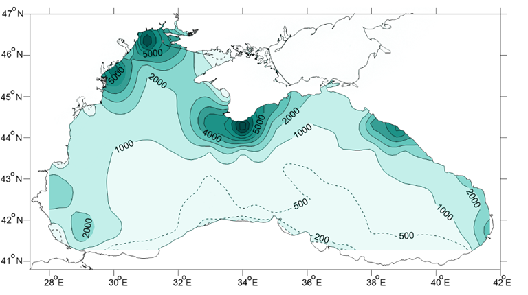
F i g. 1. Amount of oceanographic stations in the Black Sea in the 2/3° × 1° (40′ × 60′) quadrants over 1950‒2023
The methodological basis for calculating the existing climatic arrays is also different: in the SO SOI array, spline functions and standard statistical methods were used, in WOD-18 and MHI-2004 ‒ the method of successive approximations [13, 14], in MEDATLAS [15] and SeaDataNet [16] (DIVAnd ver. 2.6.4) ‒ variation inverse methods.
The calculation method of the MHI-2024 climatic array consisted of the sequential implementation of three stages.
At the first stage, the longest one, an initial array of average 10-day values for the entire observation period on a 10′ × 15′ grid was formed for regularizing the spatiotemporal heterogeneity of the initial data and filtering out mesoscale variability [17]. The optimal interpolation method [18] was used with the assumption of isotropy of the spatial correlation of thermohaline fields in the Black Sea [19, 20] and the autocorrelation function from [19]. Compared to the original data (Fig. 2, a), the interpolated data have a more uniform distribution; however, the periods before 1957 and covering 1997–2013 remain the least covered by observation data. The relative proportion of the Black Sea area covered by data in 10′ × 15′ grid nodes does not exceed 10–15% per month in these years (Fig. 3).
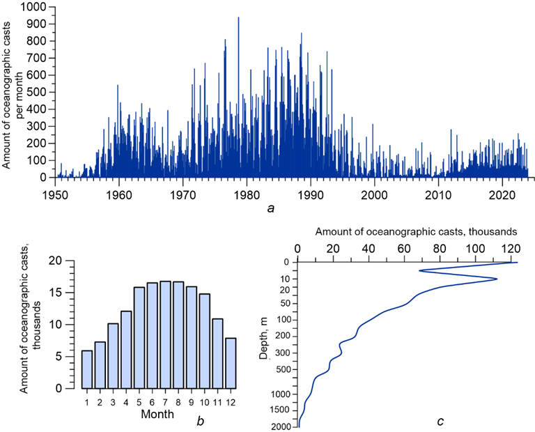
F i g. 2. Amount of oceanographic casts in the Black Sea over 1950‒2023: distribution by years and months (а), months (b) and depth (c)
At the second stage, the average monthly values for each year were calculated based on the average 10-day values at the grid nodes, then the climate average monthly values were calculated as the arithmetic means of those available for 1950‒2023.
At the third stage, the obtained average fields were smoothed by a Gaussian filter with a radius of 3‒5 grid nodes with 2‒6 iterations depending on the data availability and intraseasonal variability degree.
The resulting climatic array contains monthly average temperature and salinity fields (up to 350 m) and annual average fields (starting from 400 m) at 67 horizons: every 5 m in the 0–100 m layer with a sequential increase in the vertical step from 10 to 200 m. The climate atlas and digital array are available at the MHI ODB website (available for free access from 01.01.2025).
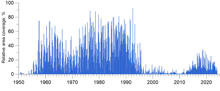
F i g. 3. Relative monthly coverage of the Black Sea water area by temperature and salinity observation data reduced to a 10´ × 15´ grid by the optimal interpolation method
T a b l e 1
Qualitative assessments of distinctions in spatial structure of water
temperature fields for February and August in the MHI-2004, WOD-18
and SeaDataNet arrays as compared to the MHI-2024 array
|
Depth, m |
Month |
MHI-2004 (1923–2004) |
WOD-18 (1981–2010) |
SeaDataNet (1955–2019) |
|
0 |
2 |
‒ |
+ |
‒ |
|
50 |
2 |
‒ |
+ |
‒ |
|
100 |
2 |
+ |
+ |
× |
|
0 |
8 |
+ |
+ |
‒ |
|
50 |
8 |
+ |
‒ |
‒ |
|
100 |
8 |
+ |
+ |
‒ |
|
500 |
8 |
‒ |
‒ |
‒ |
|
1000 |
8 |
‒ |
‒ |
+ |
Note: here and in Table 2, + means qualitative correspondence between field spatial structures and close quantitative values; × – qualitative correspondence between field spatial structures and significant difference of quantitative values; ‒ – discrepancy between field spatial structures and quantitative values.
Comparison of the MHI-2024 array with the available analogues shows that their differences in the spatial structure of hydrological fields (location of minima and maxima, seasonal configuration of cyclonic gyres) are not clearly expressed systematically as they vary by seasons and depths. Tables 1 and 2 show qualitative estimates of the differences between the arrays, using February and August as the central months of the hydrological seasons. Despite the almost identical averaging period with SeaDataNet, the MHI-2024 array is generally more similar to WOD-18 and MHI-2004, although the historical periods in them coincide only partially. Most likely, it is stipulated by the more traditional nature of the approaches used to create these arrays than SeaDataNet. Considering the fact that the set of available initial oceanographic data is almost identical due to the international exchange of hydrometeorological information, the choice of calculation methods is a determining factor for modeling the features of the spatial structure of the fields.
T a b l e 2
Qualitative assessments of distinctions in spatial structure of salinity fields
for February and August in the MHI-2004, WOD-18 and SeaDataNet arrays
as compared to the MHI-2024 array
|
Depth, m |
Month |
MHI-2004 (1923–2004) |
WOD-18 (1981–2010) |
SeaDataNet (1955–2019) |
|
0 |
2 |
+ |
+ |
+ |
|
100 |
2 |
+ |
‒ |
‒ |
|
200 |
2 |
× |
‒ |
‒ |
|
0 |
8 |
+ |
+ |
× |
|
100 |
8 |
+ |
‒ |
× |
|
200 |
8 |
+ |
‒ |
× |
|
500 |
8 |
+ |
+ |
× |
|
1000 |
8 |
‒ |
‒ |
‒ |
It is also important to consider the reliability of quantitative estimates in the deep layers of the Black Sea, where the spatiotemporal variability of thermohaline characteristics decreases sharply. The standard deviations of temperature and salinity series for the entire observation period, starting from the lower part of the main pycnocline, do not exceed 10–1 °С and salinity units, and they are within 10–3‒10–2 °С and salinity units for individual ship surveys or periods of operation of specific profiling buoys. With such homogeneity of thermohaline fields, instrumental and systematic measurement errors are comparable to natural variability, while the influence of emissions or untimely calibration of instruments increases sharply. The choice of reliable deep-sea measurement data according to metrological standards is very subjective, and strict filtering of values reduces their number necessary for reliable estimates of average values. In this regard, the spatial structure of average thermohaline fields at depths > 1000 m can be considered only as approximate one in all the arrays under consideration including MHI-2024. This also applies to average annual fields, not to mention the average monthly values presented in WOD-18 and SeaDataNet. Only vertical profiles averaged over the entire deep-water area from carefully filtered data obtained by modern measuring instruments have the greatest reliability.
It is also pertinent to highlight a further issue that frequently emerges when calculating climatic arrays. This is the formation of artificial vertical inversions, which can occur as a consequence of inconsistent spatial smoothing of fields at different horizons. When creating the MHI-2024 array, an iterative procedure for monitoring the presence of density inversions was used at the third stage of calculations, followed by an increase/decrease in the radius and the number of smoothing iterations at different horizons.
Based on the deviations of the initial data and average decadal values from the climate fields, estimates of the temporal variability intensity were calculated for different scales:
– seasonal variability  ,
,
– interannual-multidecadal variability ,
,
– mesoscale variability  ,
,
– submesoscale variability ,
,
– intraseasonal variability  , which means the total variability minus the seasonal cycle, i.e. the sum of submesoscale, mesoscale and lower-frequency (from interannual to multidecadal) variability. Here,
 –variance operator;
 – initial observation data;
 climate average monthly seasonal course;
 – monthly average anomalies,
 – mean value operator,
 – average 10-day anomalies (from the climate seasonal cycle and linear trend (at depths >100 m)),
 – average 10-day values (for 10 days),
 – climate average monthly seasonal course, approximated for each day of the year by two harmonics;
 – mesoscale anomalies,
– average 10-day anomalies (from the climate seasonal cycle and linear trend (at depths >100 m)).
Estimates of the intensity of interannual-multidecadal variability are necessary to determine the significance of long-term climate anomalies, estimates of the total intraseasonal variability help to filter measured and calculated values and estimates of mesoscale and submesoscale variability can be taken into account when studying processes of the corresponding scales.
Discussion of results
As described earlier in [21], the average vertical distribution of the estimates of the water temperature temporal variability for the Black Sea (Fig. 4, a) is characterized by one maximum: at the sea surface for the seasonal course, in the seasonal thermocline layer for the other ranges of variability. As for salinity (Fig. 4, b), all types of temporal variability have two maxima: first, at the sea surface and second, in the main halocline. Compared to [21], the estimate of the amplitude of the salinity seasonal course in the surface layer has increased as well as the estimate of the contribution of temperature and salinity submesoscale variability, which is most likely due to the fact that it was previously determined based on a fairly small number of multi-day stations. The spatial distribution of seasonal variability in the Black Sea corresponds to traditional concepts [1, 21], new estimates cover the southern part of the sea in more detail (Fig. 5).
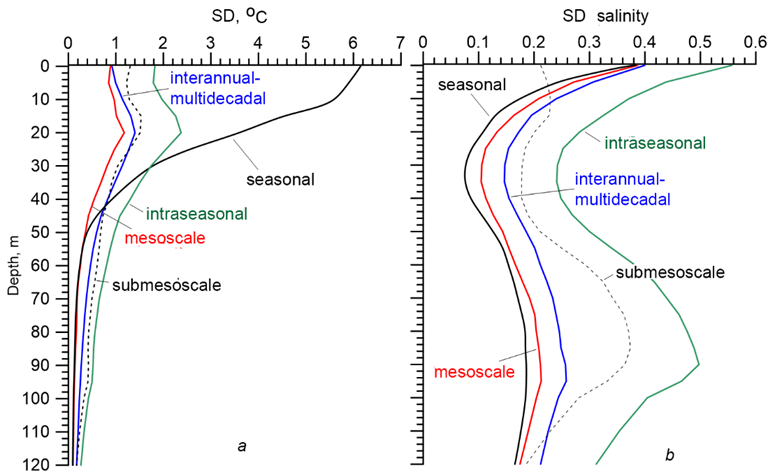
F i g. 4. Vertical distribution of the Black Sea average estimates of temporal variability of different scales for water temperature (a) and salinity (b)
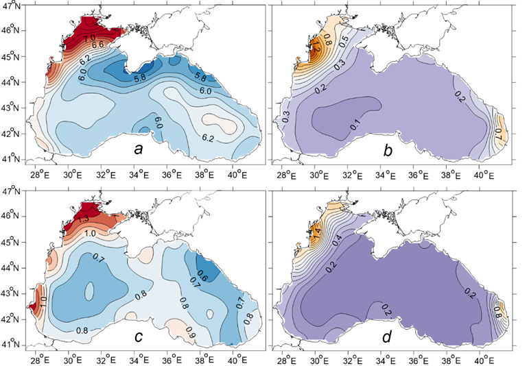
F i g. 5. Spatial distribution of temporal variability estimates on the sea surface: seasonal (a) and intraseasonal (c) water temperature SD; seasonal (b) and intraseasonal (d) salinity SD
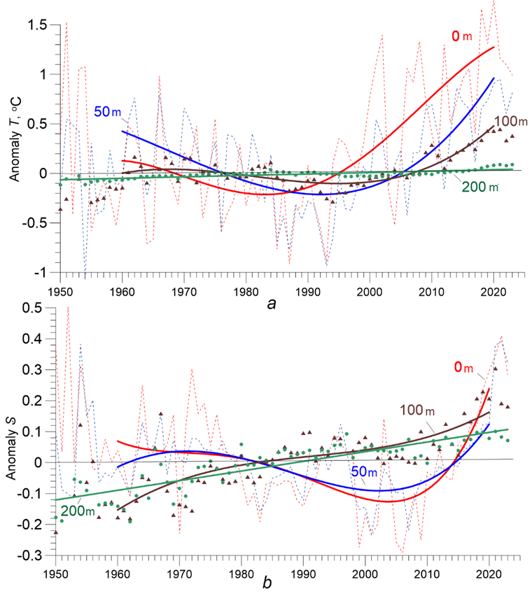
F i g. 6. Time-series of the Black Sea average annual anomalies relative to climatic seasonal values at different depths for 1950–2023: water temperature (a) and salinity (b). Thin dashed lines and symbols show anomaly values, thick lines – polynomial approximation; individual depths are highlighted in different colors
To estimate the scale of regional climate changes, average monthly and average annual temperature and salinity anomalies were calculated relative to the seasonal climate cycle at the regular grid nodes of the MHI-2024 array (Figs. 6, 7). The ratio of current anomalies to the interannual-multidecadal variability SD characterizes the relative intensity of climate changes.
After the 1980‒1990s relative cooling, positive annual average anomalies prevail in the temperature field of the Black Sea waters (Fig. 6, a). In the surface layer, the excess of the interannual SD (1.0 °C) has been observed in some years since 2000. After 2015, the warming has been steadily exceeding the average background of interannual variability. At the 50 m horizon (CIL), the excess of the interannual SD (0.6 °C) by temperature anomalies has been appearing in some years since 2010, steadily ‒ since 2015, which is often noted in the literature as the CIL going beyond the 8 °C isotherm. It should be noted that the excess of the CIL core temperature by 8 °C is not an extremely rare phenomenon as it occurred earlier at times (in the late 1930s and in 1962‒1972).
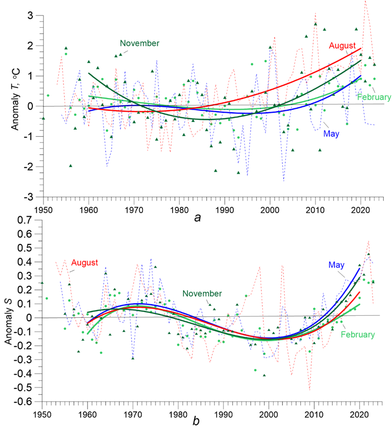
F i g. 7. Time-series of the Black Sea average monthly anomalies relative to climatic values on the sea surface in the central months of hydrological seasons for 1950–2023: water temperature (a) and salinity (b). Thin dashed lines and symbols show anomaly values, thick lines –polynomial approximation; individual months are highlighted in different colors
Also, since 2015, a stable excess of the interannual SD (0.2 °C) has been observed at the 100 m horizon. Below the 150 m depth, a stable long-term water temperature rise has been observed from the very beginning of oceanographic observations in the Black Sea. The highest seasonal increase in temperature in the surface layers occurs in summer-autumn period when the warming rate is 1.5‒2 times higher than in winter-spring one (Fig. 7, a).
After the period of surface layer freshening in the Black Sea in 1980‒2010, a sharp increase in salinity has been observed approximately from 2010–2012 (Fig. 6, b). However, the average annual anomalies do not yet exceed the interannual salinity SD (0.4) and are comparable in magnitude with the positive anomalies of 1950‒1970. The quality of salinity measurements in hydrological surveys of the 1950s can be questionable; however, measurements at coastal hydrometeorological stations also indicate high salinity values during that period.
The CIL (50 m depth) and surface layer interannual-multidecadal trends are similar, with a constant long-term increase in salinity continuing in the main halocline (≥ 75 m). The greatest seasonal increase in salinity in the surface layers takes place in spring and autumn, during the months of the positive phase of the basin water balance, indicating its general decrease and transition of the region to more arid conditions (Fig. 7, b).
Conclusion
Compared with global estimates of the 1950‒2020 climate warming rate, the linear trend of surface temperature increase in the Black Sea (0.2 °C/10 years) is generally higher than the World Ocean average trend. According to this indicator, the Black Sea belongs to areas with an increased warming rate, such as the tropical parts of the Atlantic and the Indian Ocean and the western half of the Pacific Ocean. At the same time, the Black Sea trend over a 70-year period does not reach such high values as in the Arctic seas, in the Gulf Stream-Labrador Current interaction zone or in the Falkland Current. In 1980‒2020, there was a notable rise in the surface temperature of the Black Sea amounted to 0.5 °C/10 years, second only to the trends in the Arctic regions.
Compared to global climate trends in salinity changes over 1950‒2020, the Black Sea trend in the surface layer of 0.03/10 years corresponds to positive trends in high salinity areas, in particular in large-scale subtropical gyres. Such a rate of sharp salinization as in the Black Sea in 2000‒2020 (0.18/10 years) is generally not typical for the ocean. Such rapid processes are typical of inland seas with limited external water exchange, strongly dependent on the regional freshwater balance.
In the sequence of multidecadal fluctuations in the Black Sea general hydrological state, the current warm and salty phase is similar to the 1960-1970s, but with a greater amplitude of fluctuations. Both current state and the period of 1960-1970s, in turn, follow the colder and less salty phases preceded.
1. Gertman, I.F., 1991. [Thermohaline Structure of the Black Sea]. In: A. I. Simonov and E. N. Altman, eds., 1991. Hydrometeorology and Hydrochemistry of Seas in the USSR. Vol. 4. Black Sea. Issue 1. Hydrometeorological Conditions. St. Petersburg: Gidrometeoizdat, pp. 146-195 (in Russian).
2. Locarnini, R.A., Mishonov, A.V., Baranova, O.K., Boyer, T.P., Zweng, M.M., Garcia, H.E., Reagan, J.R., Seidov, D., Weathers, K.W. [et al.], 2019. World Ocean Atlas 2018. Volume 1: Temperature. Silver Spring, MD, USA: NOAA Atlas NESDIS, 52 p.
3. Zweng, M.M., Reagan, J.R., Seidov, D., Boyer, T.P., Locarnini, R.A., Garcia, H.E., Mishonov, A.V., Baranova, O.K., Weathers, K.W. [et al.], 2019. World Ocean Atlas 2018. Volume 2: Salinity. Silver Spring, MD, USA: NOAA Atlas NESDIS, 50 p.
4. Suvorov, A.M., Palmer, D.R., Khaliulin, A.K., Godin, E.A. and Belokopytov, V.N., 2003. Digital Atlas and Evaluation of the Influence of Inter-Annual Variability on Climate Analyses. In: Oceans 2003. Celebrating the Past… Teaming Toward the Future. San Diego, CA, USA: IEEE. Vol. 2, pp. 990-995. https://doi.org/10.1109/OCEANS.2003.178468
5. Polonsky, A.B., Shokurova, I.G. and Belokopytov, V.N., 2013. Decadal Variability of Temperature and Salinity in the Black Sea. Morskoy Gidrofizicheskiy Zhurnal, (6), pp. 27-41 (in Russian).
6. Miladinova, S., Stips, A., Garcia-Gorriz, E. and Macias Moy, D., 2017. Black Sea Thermohaline Properties: Long-Term Trends and Variations. Journal of Geophysical Research: Oceans, 122(7), pp. 5624-5644. https://doi.org/10.1002/2016JC012644
7. Polonsky, A.B. and Serebrennikov, A.N., 2023. Changes in the Nature of Temperature Anomalies of the Black Sea Surface during the Warming Period of the Late 20th – Early 21st Centuries. Issledovanie Zemli iz Kosmosa, (6), pp. 118-132. https://doi.org/10.31857/S0205961423060064 (in Russian).
8. Belokopytov, V.N., 2011. Interannual Variations of the Renewal of Waters of the Cold Intermediate Layer in the Black Sea for the Last Decades. Physical Oceanography, 20(5), pp. 347-355. https://doi.org/10.1007/s11110-011-9090-x
9. Capet, A., Troupin, C., Carstensen, J., Grégoire, M. and Beckers, J.-M., 2014. Untangling Spatial and Temporal Trends in the Variability of the Black Sea Cold Intermediate Layer and Mixed Layer Depth Using the DIVA Detrending Procedure. Ocean Dynamics, 64(3), pp. 315-324. https://doi.org/10.1007/s10236-013-0683-4
10. Miladinova-Marinova, S., Stips, A., Garcia Gorris, E. and Macias Moy, D., 2018. Formation and Changes of the Black Sea Cold Intermediate Layer. Progress in Oceanography, 167, pp. 11-23. https://doi.org/10.1016/j.pocean.2018.07.002
11. Stanev, E.V., Peneva, E. and Chtirkova, B., 2019. Climate Change and Regional Ocean Water Mass Disappearance: Case of the Black Sea. Journal of Geophysical Research: Oceans, 124(7), pp. 4803-4819. https://doi.org/10.1029/2019JC015076
12. Polonskii, A.B. and Novikova, A.M., 2020. Interdecadal Variability of the Black Sea Cold Intermediate Layer and Its Causes. Russian Meteorology and Hydrology, 45(10), pp. 694-700. https://doi.org/10.3103/S1068373920100039
13. Cressman, G.P., 1959. An Operational Objective Analysis System. Monthly Weather Review, 87(10), pp. 367-374. https://doi.org/10.1175/1520-0493(1959)087<0367:AOOAS>2.0.CO;2
14. Barnes, S.L., 1964. A Technique for Maximizing Details in Numerical Weather Map Analysis. Journal of Applied Meteorology and Climatology, 3(4), pp. 396-409. https://doi.org/10.1175/1520-0450(1964)003<0396:ATFMDI>2.0.CO;2
15. Rixen, M., Beckers, J.-M., Brankart, J.-M. and Brasseur, P., 2000. A Numerically Efficient Data Analysis Method with Error Map Generation. Ocean Modelling, 2(1-2), pp. 45-60. https://doi.org/10.1016/S1463-5003(00)00009-316
16. Barth, A., Beckers, J.-M., Troupin, C., Alvera-Azcàrate, A. and Vandenbulcke, L., 2014. DIVAnd-1.0: n-Dimensional Variational Data Analysis for Ocean Observations. Geoscientific Model Development, 7(1), pp. 225-241. https://doi.org/10.5194/gmd-7-225-2014
17. Belokopytov, V.N., 2018. Retrospective Analysis of the Black Sea Thermohaline Fields on the Basis of Empirical Orthogonal Functions. Physical Oceanography, 25(5), pp. 380-389. https://doi.org/10.22449/1573-160X-2018-5-380-389
18. Bretherton, F.P., Davis, R.E. and Fandry, C.B., 1976. A Technique for Objective Analysis and Design of Oceanographic Experiments Applied to MODE-73. Deep Sea Research and Oceanographic Abstracts, 23(7), pp. 559-582. https://doi.org/10.1016/0011-7471(76)90001-2
19. Grigor’ev, A.V., Ivanov, V.A. and Kapustina, N.A., 1996. Correlation Structure of the Black Sea Thermohaline Fields in the Summer Season. Oceanology, 36(3), pp. 334-339.
20. Polonskii, A.B. and Shokurova, I.G., 2008. Statistical Structure of the Large-Scale Fields of Temperature and Salinity in the Black Sea. Physical Oceanography, 18(1), pp. 38-51. https://doi.org/10.1007/s11110-008-9008-4
21. Ivanov, V.A. and Belokopytov, V.N., 2013. Oceanography of the Black Sea. Sevastopol: ECOSI-